Equivariance and Invariance for Robust Unsupervised and Semi-Supervised Learning

(1)

University of Central Florida University of Central Florida

STARS

Electronic Theses and Dissertations, 2020-

2020

Equivariance and Invariance for Robust Unsupervised and

Semi-Supervised Learning

Supervised Learning

Liheng Zhang

University of Central Florida

Part of the Computer Sciences Commons

Find similar works at: https://stars.library.ucf.edu/etd2020 University of Central Florida Libraries http://library.ucf.edu

This Doctoral Dissertation (Open Access) is brought to you for free and open access by STARS. It has been accepted for inclusion in Electronic Theses and Dissertations, 2020- by an authorized administrator of STARS. For more information, please contact [email protected].

STARS Citation STARS Citation

Zhang, Liheng, "Equivariance and Invariance for Robust Unsupervised and Semi-Supervised Learning" (2020). Electronic Theses and Dissertations, 2020-. 159.

(2)

EQUIVARIANCE AND INVARIANCE FOR ROBUST UNSUPERVISED AND SEMI-SUPERVISED LEARNING

by

LIHENG ZHANG

B.S. Huazhong University of Science and Technology, 2015

A dissertation submitted in partial fulfilment of the requirements for the degree of Doctor of Philosophy

in the Department of Computer Science in the College of Engineering and Computer Science

at the University of Central Florida Orlando, Florida

Spring Term 2020

(3)

c

(4)

ABSTRACT

Although there is a great success of applying deep learning on a wide variety of tasks, it heavily relies on a large amount of labeled training data, which could be hard to obtain in many real scenar-ios. To address this problem, unsupervised and semi-supervised learning emerge to take advantage of the plenty of cheap unlabeled data to improve the model generalization. In this dissertation, we claim that equivariant and invariance are two critical criteria to approach robust unsupervised and semi-supervised learning. The idea is as follows: the features of a robust model ought to be sufficiently informative and equivariant to transformations on the input data, and the classifiers should be resilient and invariant to small perturbations on the data manifold and model parameters. Specifically, features are learnt via auto-encoding the transformations on the input data, and models are regularized through minimizing the effects of perturbations on features or model parameters. Experiments on several benchmarks show the proposed methods outperform many state-of-the-art approaches on unsupervised and semi-supervised learning, proving importance of the equivariance and invariance rules for robust feature representation learning.

(5)

(6)

ACKNOWLEDGMENTS

I would like to gratefully thank my academic advisors Dr. Guo-Jun Qi and Dr. Liqiang Wang. I also want to thank my advisory committee members, Dr. Ulas Bagci and Dr. Fei Liu for their time and comments.

I would also like to thank my labmates, Hao Hu, Zihang Zou and Marzieh Edraki for friendship and communications for interesting ideas. Special thanks to my parents, my sister and my brother in law for supporting me during the past five years.

(7)

LIST OF FIGURES

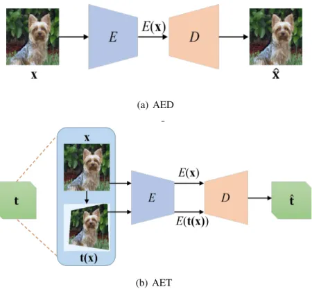
Figure 3.1: An illustrative comparison between AED and AET . . . 12

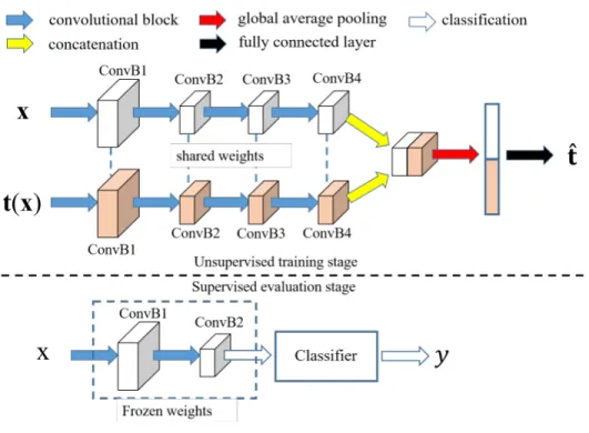
Figure 3.2: An illustration of the network architectures for training and evaluating AET on the CIFAR-10 dataset. . . 18

Figure 3.3: The comparison of the KNN error rates by different models with varying numbers K of nearest neighbors on CIFAR-10. . . 22

Figure 3.4: Error rate (top-1 accuracy) vs. AET loss over epochs on the CIFAR-10 and ImageNet datasets. . . 26

Figure 3.5: Some examples of predicted transformations by the AET. . . 27

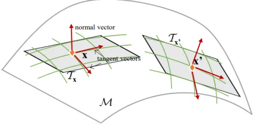
Figure 4.1: Illustration of a curved manifold M embedded in 3- dimensional ambient space. . . 30

Figure 4.2: Network architecture for local generators on the CelebA dataset. . . 40

Figure 4.3: Faces generated by LGAN on the CelebA dataset. . . 41

Figure 4.4: Handwritten digits generated by LGAN on the MNITS dataset. . . 42

Figure 4.5: Network architecture for local generators on SVHN and CIFAR-10. . . 43

Figure 4.6: Tangent images generated by LGAN along ten randomly chosen coordinates on SVHN and CIFAR-10 datasets. . . 45

(12)

Figure 5.1: (a) A toy example of a sigmoid unit for four datapoints; (b) the relation be-tweenφand the corresponding WCP value. . . 47

(13)

LIST OF TABLES

Table 3.1: Comparison between unsupervised feature learning methods on CIFAR-10. . 20

Table 3.2: Error rates of different classifiers on CIFAR 10. . . 22

Table 3.3: ImageNet top-1 classification with non-linear layers . . . 24

Table 3.4: ImageNet top-1 classification with linear layers. . . 25

Table 3.5: Places top-1 classification with linear layers. . . 26

Table 4.1: Classification errors on both SVHN and CIFAR-10 datasets compared with the state-of-the-art methods. . . 44

Table 5.1: Error rate on CIFAR-10 over ten runs with different number of labeled ex-amples. All methods use the same 13-layer architecture. . . 58

Table 5.2: Error rate on SVHN over ten runs with different number of labeled examples. All methods use the same 13-layer architecture. . . 58

Table 5.3: Ablation study of the impact of different model components. The error rate is reported on the test set of CIFAR-10 with4,000labels. . . 59

Table 5.4: Error rate of worst-case dropconnect perturbations on different layers of each convolutional block on CIFAR-10 with4,000labels. . . 59

Table 5.5: Error rate of the WCP with different dropconnect ratios on CIFAR-10 with 4,000labels, with the other hyperparameters fixed. . . 59

(14)

CHAPTER 1: INTRODUCTION

1.1 Motivation

Deep learning has achieved a tremendous success recent years in a wide variety of tasks, such as image classification [13], object detection [54, 53] and semantic segmentation [34, 66]. How-ever, its success usually requires a huge amount of labeled training data to learn adequate feature representations. For example, millions of images are collected and labeled to train a1,000-way classifier on the ImageNet dataset [13]. Unfortunately, such a large scale of labeled data are usu-ally difficult to obtain in many real scenarios, limiting the applicability of deep neural networks. Thus, it arises the research interests in literature on unsupervised and semi-supervised learning to address the problem of training with insufficient labeled data.

In this dissertation, we formalize the equivariance and invariance [24, 9, 50] as critical criteria on robust unsupervised and semi-supervised learning. Formally, Given an inputxand a function f, functionf is equivariant to a transformation tiff(t(x)) = t(f(x)). In other words, applying the transformationt onxequivary to applying it on the output f(x). On the other hand, iff(t(x)) =

f(x), functionf is invariant againsttsince applyington the input does not change the output.

Despite lacking of solid theories, it is thought that Convolutional Neural Networks (CNNs) benefit from both translation equivariance and invariance [9, 10, 24]. Typically, a CNN usually comprises of two parts: feature maps from multiple convolutional layers and a classifier with fully connected layers mapping the feature maps into labels. It is obvious that the convolutional feature maps are equivariant with respect to translations as they shift in the same way as the input images with convolution and padding. On the contrary, by minimizing the classification loss on examples aug-mented with translations, the classifier obtains the translation invariance property as it predicts the

(15)

translated image with the same label as the original image. Motivated by this, it is natural to extend this idea by generalizing translations to other forms of transformations, e.g. affine transformations, projective transformations and even GAN-induced transformations.

To achieve equivariance to transformations, we propose to learn unsupervised feature representa-tions via Auto-Encoding Transformarepresenta-tions (AET) [68] on the input images. In this way, features encoding the visual structure of the images are sufficiently informative to predict the transforma-tions.

Moreover, we investigate the invariance against GAN-induced transformations specifically. A Lo-calized Generative Adversarial Network (LGAN) [49] is proposed to access the local geometry of the data manifold and generate local images by adding random perturbations on the feature space. Regarding the LGAN as a transformation function, the classifier is regularized to make smooth predictions with the local images, so as to be invariant against perturbations on the data manifold.

Beyond transformations on the input data, we further extend the definition of the invariance in the case of perturbations on model parameters. For a classifierfθ with parametersθ, we consider

a perturbation g on θ instead of on the input data x. Thus, the invariance rule is re-defined as

fθ(x) = fg(θ)(x). Through minimizing the efforts of Worst-Case Perturbations (WCP) [67], the classifier makes stable predictions for both labeled and unlabled data.

1.2 Contributions

Per equivariance to transformations, e.g. affine transformations and projective transformations, we will present a novel paradigm of unsupervised representation learning by Auto-Encoding Trans-formation (AET) [68] in contrast to the conventional Auto-Encoding Data (AED) approach. Given a randomly sampled transformation, AET seeks to predict it merely from the encoded features

(16)

as accurately as possible at the output end. The idea is the following: as long as the unsuper-vised features successfully encode the essential information about the visual structures of original and transformed images, the transformation can be well predicted. We will show that this AET paradigm allows us to instantiate a large variety of transformations, from parameterized, to non-parameterized and GAN-induced ones. Our experiments show that AET greatly improves over existing unsupervised approaches, setting new state-of-the-art performances being greatly closer to the upper bounds by their fully supervised counterparts on CIFAR-10 [29], ImageNet [13] and Places [72] datasets.

With perturbations on the manifold of real data, we also propose a novel Localized Generative Adversarial Net (LGAN) [49] for the invariance principle. Compared with the classic GAN that globally parameterizes a manifold, the Localized GAN (LGAN) uses local coordinate charts to parameterize distinct local geometry of how data points can transform at different locations on the manifold. Specifically, around each point there exists a local generator that can produce data following diverse patterns of transformations on the manifold. The locality nature of LGAN en-ables local generators to adapt to and directly access the local geometry without need to invert the generator in a global GAN. Furthermore, it can prevent the manifold from being locally col-lapsed to a dimensionally deficient tangent subspace by imposing an orthonormality prior between tangents. This provides a geometric approach to alleviating mode collapse at least locally on the manifold by imposing independence between data transformations in different tangent directions. We will demonstrate the LGAN can be applied to train a robust classifier that prefers locally con-sistent classification decisions on the manifold, yielding the perturbation invariance. The resultant regularizer is closely related with the Laplace-Beltrami operator. Our experiments show that the proposed LGANs can not only produce diverse image transformations, but also deliver superior classification performances.

(17)

the Worse-Case Perturbation (WCP) [67] on model parameters to achieve perturbation invariance. It is based on the idea that a robust model is least likely to be affected by small perturbations, such that its output decisions should be as stable as possible on both labeled and unlabeled examples. We will consider two forms of WCP regularizations – additive and DropConnect perturbations, which impose additive noises on network weights, and make structural changes by dropping the network connections, respectively. We will show that the worse cases of both perturbations can be derived by solving respective optimization problems with spectral methods. The WCP can be minimized on both labeled and unlabeled data so that networks can be trained in a semi-supervised fashion. This leads to a novel paradigm of semi-supervised classifiers by stabilizing the predicted outputs in presence of the worse-case perturbations imposed on the network weights and structures. We conduct experiments to demonstrate the proposed method outperforms many state-of-the-art models in literature.

1.3 Outline

This dissertation is organized as follows.

Chapter 1 introduces the background of unsupervised and semi-supervised learning, and illustrates the motivations and contributions of this dissertation.

Chapter 2 presents related works in literature on the unsupervised and semi-supervised learning topics.

Chapter 3 proposes a method called Auto-encoding Transformations (AET) to achieve robust unsu-pervised learning. Transformations are adopted on the image data. We will show the equivariance as a critical criterion on feature representation learning.

(18)

Chapter 4 shows details of perturbing on the data manifold. A Localized GAN model is presented to generate local images and train robust classifiers resilient and invariant to these perturbations.

Chapter 5 proposes a method called Worst-Case Perturbation on model parameters for semi-supervised learning, so as to demonstrate that the perturbation invariance principle yields robust classifiers with stable predictions.

(19)

CHAPTER 2: RELATED WORK

2.1 Unsupervised Learning

Auto-Encoders. The use of auto-encoder architecture in learning representations in an unsuper-vised fashion has been extensively studied in literature [23, 25, 63]. These existing auto-encoders are all based on reconstructing the input data at the output end through a pair of encoder and decoder. The encoder acts as an extractor of features usually compactly representing the most essential information about input data, while a decoder is jointly trained to recover the input data upon the extracted features. The idea is that a good feature representation should contain suf-ficient information to reconstruct the input data. A wide spectrum of auto-encoders have been proposed following this paradigm of encoding data (AED). For example, the variational auto-encoder [26] explicitly introduces probabilistic assumption about the distribution of features ex-tracted from data. Denoising auto-encoder [63] aims to learn more robust representation by re-constructing original inputs from noise-corrupted inputs. Contrastive AutoEncoder [55] penalizes abrupt changes of representations around given data, thus encouraging representation invariance to small perturbation on input data. Zhang et al. [70] present a cross-channel auto-encoder by reconstructing a subset of data channels from another subset with the crosschannel features being concatenated as data representation. Hinton et al. [24] propose a transforming auto-encoder in the context of capsule nets, which is still trained in the AED fashion by minimizing the discrepancy between the reconstructed and target images.

Generative Adversarial Nets. Besides the auto-encoders, Generative Adversarial Nets (GANs) become popular for training network representations of data in an unsupervised fashion. Unlike the auto-encoders, GANs attempt to directly generate data from noises drawn from a random dis-tribution. By viewing the sampled noises as the coordinates over the manifold of real data, one

(20)

can use them as the features to represent data. For this purpose, one usually needs to train a data encoder to find the noise that can generate the input images through the GAN generator. This can be implemented by jointly training a pair of mutually inverse generator and encoder [15, 17]. A prominent characteristic of GANs that make them different from auto-encoders is they do not rely on one-to-one reconstruction of input data at the output end. Instead, they focus on discovering and generating the entire distribution of data over the underlying manifold. Recent progress has shown the promising generalization ability of regularized GANs in generating unseen data based on the Lipschitz assumption on the real data distribution [46, 2], and this shows great potential of GANs in providing expressive representation of images [15, 17, 18].

Self-Supervised Representation Learning. In addition to auto-encoders and GANs, other unsu-pervised learning methods explore various self-suunsu-pervised signals to train deep neural networks. These self-supervised signals can be directly derived from data themselves without having to be manually labeled. For example, Doersch et al. [14] use the relative positions of two randomly sampled patches from an image as self-supervised information to train the model. Mehdi and Favaro [38] propose to train a convolutional neural network by solving Jigsaw puzzles. Noroozi et al. [39] learn counting features that satisfy equivalence relations between downsampled and tiled images, and Gidaris et al. [20] train neural networks by classifying image rotations in a discrete set. Dosovitskiy et al. [16] train CNNs by classifying a set of surrogate classes, each of which is formed by applying various transformations to an individual image. However, the resultant fea-tures could over-discriminate visually similar images as they always belong to different surrogate classes, and the training cost is much more expensive as every training example results in an in-dividual surrogate class. Luo et al. [35] introduce the concept of image-transform bootstrapping using transforms in the image space to augment training, testing, and both. The idea has also been employed to train feature representations for videos through the self-motion of moving objects [1]. In summary, this type of approaches train networks using various self-supervised objectives

(21)

instead of manually labeled data.

In Chapter 3, we will present an alternative paradigm of unsupervised learning, Auto-Encoding Transformations (AET) [68], motivated by transformation equivariance. Conceptually, the Auto-Encoders differ from the proposed AET that aims to learn unsupervised features by directly min-imizing the input and output transformations in an end-to-end auto-encoder architecture. Without restrictions of the transformation forms, the AET framework explore dynamics of features with dif-ferent transformations instead of the static representations learnt by auto-encoders, so as to reveal the intrinsic visual structures of the images.

2.2 Semi-supervised Learning

Generative Adversarial Networks.Besides unsupervised feature representation learning, another important applications of GANs lies in the classification problem, especially considering their ability of modeling the manifold structures for both labeled and unlabeled examples in a semi-supervised fashion [59, 60, 48]. For example, [27] presented variational autoencoders [26] by combining deep generative models and approximate variational inference to explore both labeled and unlabeled data. [56] treated the samples from the GAN generator as a fake class, and explore unlabeled examples by assigning them to a real class different from the fake one. [52] proposed to train a ladder network [62] by minimizing the sum of supervised and unsupervised cost functions through back-propagation, which avoids the conventional layer-wise pre-training approach. [58] presented an approach to learning a discriminative classifier by trading-off mutual information between observed examples and their predicted classes against an adversarial generative model. [17] sought to jointly distinguish between not only real and generated samples but also their latent variables in an adversarial fashion. [12] presented to train a semi-supervised classifier by exploring the areas where real samples are unlikely to appear.

(22)

In Chapter 4, we will explore the ability of the Localized GANs (LGANs) [49] to model the data distribution and its manifold geometry to train a robust classifier, which can make locally consis-tent classification decisions in presence of small perturbations on the feature space. The idea of training a locally consistent classifier could trace back almost two decades ago to TangentProp [57] that pursued classification invariance against image rotation and translation manually performed in an ad-hoc fashion. Kumar et al. [31] extended the TangentProp by training an augmented form of BiGAN to explore the underlying data distributions, but it still relied on a global GAN to indirectly access the local tangents by learning a separate encoder network. On the contrary, the local co-ordinates will enable the LGAN to directly access the geometry of image transformations to train a locally consistent classifier, along with the orthonormality between local tangents allowing the learned classifier to explore its local consistency against independent image transformations along different local coordinates on the manifold.

Corrupting the Models.There also exist several works in literature that regularize the model train-ing by randomly corrupting networks. Among them is the seminal dropout regularization that randomly removes neurons when training networks [30]. Along this line, the DropConnect [64] is a natural extension by randomly dropping neural connections during the training. Essentially, the removal of neurons and their connections can be seen as forming an ensemble of network architectures in the training process, yielding a robust network by “averaging” over the resultant ensemble.

This idea has been further extended to train semi-supervised classifiers by temporally fusing net-works through the training process. For example, [32] propose to predict target values of unlabeled examples by taking an exponential moving average of the predictions from stochastic networks trained with random dropouts and data augmentations over recent iterations. [61] further extend the idea of the temporal ensembling to maximize the consistency of predictions between mean teachers and the running student networks on both labeled and unlabeled data.

(23)

Instead of generating an ensemble ofrandomly corrupted networks, the Worst-Case Perturbation (WCP) [67] in Chapter 5 aims to find and enhance the most vulnerable part of a network by making the weights and connections most resilient against the worst-case perturbations. In contrast to the WCP that directly imposes perturbations on network weights and structures, [36] explore the vulnerability of a network through virtual adversarial examples that would maximally alter the network predictions. The WCP is orthogonal to the approach that uses the virtual adversarial examples to train a robust classifier [36]. In contrast, the WCP seeks to reveal and enhance the most vulnerable part of the model in terms of both additive and dropconnect noises. As aforementioned, the WCP is also well connected with the idea of training robust models with the large margin principle [6, 11] that has gained success before the deep learning era. Thus, we also aim to close the research gap by bringing the principle of classic regularization methods to train more competitive deep networks.

(24)

CHAPTER 3: EQUIVARIANCE TO TRANSFORMATIONS ON INPUT

DATA

In this chapter, we present a noval paradigm of Auto-Encoding Transformations (AET) [68] for unsupervised learning to learn informative features representations that equivary to transformations on the input data. We demonstrate the importance of Transformation Equivariance Representations (TERs) on unsupervised learning.

Among the efforts on unsupervised learning methods, the most representative ones are Auto-Encoders and Generative Adversarial Nets (GANs) [22]. The former trains an encoder network to output feature representations with sufficient information to reconstruct input images by a paired decoder. Many variants of auto-encoders [24, 26] have been proposed in literature but all of them stick to essentially the same idea of reconstructing input data at the output end, and thus we classify them into the Auto-Encoding Data (AED) paradigm illustrated in Figure 3.1(a).

On the other hand, GANs learn the feature representation in an unsupervised fashion by generating images from input noises with a pair of adversarially trained generator and discriminator. The input noises into the generator can be viewed as the feature representations of its output, since they contain necessary information to produce the corresponding images through the generator. To obtain the “noise” feature representation for each image, an encoder can be trained to form an auto-encoder architecture with the generator as the decoder. In this way, given an input image, the encoder can directly output its noise representation producing the original image through the generator [15, 17]. This combines the strength of both AED and GAN models. Recently, these models become a popular alternative to autoencoders in many unsupervised and semi-supervised tasks, as they can generate the distribution of photo-realistic images as a whole so that better feature representations can be derived from the trained generator.

(25)

(a) AED

(b) AET

Figure 3.1: An illustrative comparison between AED and AET

Besides auto-encoders and GANs, various paradigms of self-supervised learning methods exist without using manually labeled data. These methods create self-supervised objectives to train the networks. For example, Doersch et al. [14] propose to train neural networks by predicting the relative positions of two randomly sampled patches. Mehdi and Favaro [38] report to train a convolutional neural network by solving Jigsaw puzzles. Image colorization has also been used as a self-supervised task to train convolutional networks in literature [69, 33]. Instead, Dosovitskiy et al. [16] train neural networks by discriminating among a set of surrogate classes artificially formed by applying various transformations to image patches, while Gidaris et al. [20] attempt to classify image rotations of four discrete angles. These approaches explore supervisory signals at various levels of visual structures to train networks without manually labeling data. Unsupervised features have also been extracted from videos by estimating the self-motion of moving objects between

(26)

consecutive frames [1].

In contrast, we are motivated to learn unsupervised feature representations by Auto-Encoding Transformations (AET) rather than the data themselves. Specifically, by sampling some opera-tors to make transformations on images, we seek to train auto-encoders that can directly recon-struct these operators from the learned feature representations between original and transformed images. We believe as long as the trained features are sufficiently informative and equivariant to such transformations, we can decode the transformations from the features that well encode visual structures of images. As compared with the conventional paradigm of Auto-Encoding Data (AED) in Figure 3.1, AET focuses on exploring dynamics of feature representations under different trans-formations, thereby revealing not only static visual structures but also how they would change by applying different transformations. Moreover, there is no restriction on the form of transformations applicable in the proposed AET framework. This allows us to flexibly explore a large variety of transformations, ranging from simple image warping to any parametric and nonparametric transfor-mations. We will demonstrate the AET representations outperform the other unsupervised models in experiments, greatly pushing the state-of-the-art unsupervised method much closer to the upper bound set by the fully supervised counterparts.

3.1 AET: The Proposed Approach

We elaborate on the proposed paradigm of autoencoding transformations (AET) in this section. First, we will formally present the formulation of AET in Section 3.1.1 Then we will instantiate AET with different genres of transformations in Section 3.1.2.

(27)

3.1.1 The Formulation

Suppose that we sample a transformationt from a distributionT (e.g., image warping, projective transformation and even GAN-induced transformation, c.f. Section 3.1.2 for more details). It is applied to an imagexdrawn from a data distributionX, resulting in the transformed versiont(x)

ofx.

Our goal is to learn an encoderE : x →E(x), which aims to extract the representationE(x)for a sample x. Meanwhile, we wish to learn a decoder D : [E(x), E(t(x))] → ˆ_t_{, which gives an}

estimatetˆof input transformation by decoding from the encoded representations of original and transformed images. Since the prediction on the input transformation is made through the encoded features rather than the original and transformed images, it forces the model to extract expressive features as a proxy to represent images.

The learning problem of Auto-Encoding Transformations (AET) now boils down to jointly training the feature encoderEand the transformation decoderD. To this end, let us choose a loss function

`(t,ˆ(t))that quantifies the difference between a transformationtand its estimateˆt. Then the AET can be solved by minimizing this loss as

min

E,D t∼TE,x∼X`(t, ˆ

t)

where the transformation estimateˆtis a function of the encoderE and the decoderDsuch that

ˆ

t=D[E(x), E(t(x))],

and the expectationE is taken over the sampled transformations and data. Like in training other

(28)

by back-propagating the gradient of the loss`.

3.1.2 The AET Family

A large variety of transformations can be easily incorporated into the AET formulation. Here we discuss three genres, parameterized, GAN-induced and non-parameterized transformations, to instantiate the AET models.

Parameterized Transformations. Suppose that we have a family of transformationsT ={tθ|θ ∼ Θ}with their parametersθsampled from a distributionΘ. This equivalently defines a distribution of parameterized transformations, where each transformation can be represented by its parameter and the loss`(tθ, t_θˆ)between transformations can be captured by the difference in terms of their parameters. For example, many transformations such as affine and projective transformations can be represented by a parameterized M(θ) ∈ _R3×3 _{between homogeneous coordinates of images} before and after transformations. Such a matrix captures the change of geometric structures caused by a given transformation, and thus it is straightforward to`(tθ, t_θˆ) = 1₂||M(θ)−M(ˆθ)||22to model the difference between the target and the estimated transformations. In the experiments, we will compare different instances of parameterized transformations in this category and demonstrate they can yield competitive performances on training AET.

GAN-Induced Transformations.One can choose other forms of transformations without explicit geometric implications like the affine and the projective transformations. Let us consider a GAN generator that transforms an input over the manifold of real images. For example, in [49], a lo-cal generatorG(x, z)is learned with a sampled random noisez that parameterizes the underlying transformation around a given image x. This effectively defines a GANinduced transformation such thattz(x) = G(x, z)with the transformation parameterz. One can directly choose the loss

(29)

from the featuresE(x)andE(tz(x))by the encoder networkE. Compared with the classical

trans-formations that change low-level appearance and geometric structures in images, the GAN-induced transformations can change high-level semantics in images. For example, the GANs have demon-strated their ability of manipulating attributes such as ages, hairs, genders and wearing glasses in facial images as well as changing the furniture layout in bedroom images [51]. This enables AET to explore a richer family of transformations to learn more expressive representations.

Non-Parametric Transformations. Even if a transformation t ∈ T is hard to parameterize, we can still define the loss`(t,ˆt)by measuring the average difference between the transformations of randomly sampled images. Formally,

`(t,ˆt) = _E x∼X

dist(t(x),ˆt(x)) (3.1)

wheredist(·,·)is a distance between two transformed images, and the expectation is taken over random samples. For an input non-parametric transformationt, we also need a decoder network that outputs a transformationˆtto estimate the input transformation. This can be done by choosing a parameterized transformationt_θˆasˆtto estimatet. Although the non-parametrictmay not fall in the space of parameterized transformations, such an approximation should be enough for unsupervised learning since our ultimate goal is not to obtain an accurate estimate of input transformation; instead, we aim at learning a good feature representation to give us the best estimate that can be achieved in the parameterized transformation space.

Note that parameterized transformations can also be plugged into Eq. 3.1 to train the corresponding AET by minimizing this loss function. However, in experiments, we find the performance is not as good as the AET trained with the parameter-based loss. This is probably caused by the fact that the loss 3.1 cannot accurately reflect the actual difference between transformations unless a sufficiently large number of images are sampled. Thus, we suggest using the parameter-based

(30)

loss for the AET with parameterized transformations. We have shown that a wide spectrum of transformations can be adopted in training AET. In this chapter, we will focus on the parameterized transformations as they do not involve training extra models like GAN-induced transformations, or require choosing auxiliary transformations to approximate non-parametric forms. This allows us to make a straightforward and fair comparison with the unsupervised methods in literature as shown in the experiments. Moreover, the GAN-induced transformations greatly rely on the quality of transformed images, but existing GAN models are still unable to generate high-quality images with fine-grained details at a high resolution. Thus, we leave it in future to study the GAN-induced and non-parametric transformations for training the AET representations.

3.2 Experiments

In this section, we evaluate the proposed AET model on the CIFAR-10, ImageNet and Places datasets by comparing it against different unsupervised methods. Unsupervised learning is usually evaluated indirectly based on the classification performance by using the learned representations. For the sake of fair comparison, we follow the test protocols widely adopted in literature.

3.2.1 CIFAR-10 Experiments

First, we evaluate the AET model on the CIFAR-10 dataset. We consider two different transfor-mations – affine and projective transfortransfor-mations – to train AET, and name the resultant models AET-affine and AET-project for brevity, respectively.

(31)

3.2.1.1 Architecture and Implementation Details

To make a fair and direct comparison with existing unsupervised models, we adopt the Network-In-Network (NIN) architecture that has shown competitive performance previously on the CIFAR-10 dataset for the unsupervised learning task [20]. As illustrated in the top of Figure 2, the NIN con-sists of four convolutional blocks, each of which contains three convolutional layers. AET has two NIN branches, each taking the original and the transformed images as its input, respectively. The output features of the forth block of two branches are concatenated and averagepooled to form a 384-d feature vector. Then an output layer follows to predict the parameters of input transfor-mation. The two branches share the same network weights, and are used as the encoder network producing the feature representations for input images.

Figure 3.2: An illustration of the network architectures for training and evaluating AET on the CIFAR-10 dataset.

(32)

trans-formed counterparts. Momentum and weight decay are set to0.9and5×10−4_{. The learning rate is} initialized to0.1and scheduled to drop by a factor of5after240,480,640,800and1,000epochs. The model is trained for1,500epochs in total. For AET-affine, the affine transformation is a com-position of a random rotation with [−180◦,180◦], a random translation by±0.2of image height and width in both vertical and horizontal directions, and a random scaling factor of[0.7,1.3], along with a random shearing of[−30◦,30◦]degree. For the AET-projective, the projective transforma-tion is formed by randomly translating four corners of an image in both horizontal and vertical directions by ±0.125 of its height and width, after it is randomly scaled by[0.8,1.2]and rotated by 0◦, 90◦, 180◦ or 270◦. We compare the results for both models below, and demonstrate both outperform the other existing models and AET-project performs better than AET-affine.

3.2.1.2 Evaluation Protocol

To evaluate the quality of the representation by an unsupervised model, a classifier is usually trained upon the learned features. Specifically, in our experiments on CIFAR-10, we follow the existing evaluation protocols [41, 16, 51, 20] by building a classifier on top of the second convolu-tional block. See the bottom of Figure 3.2, where the first two blocks are frozen while the classifier on top of them is trained with labeled examples.

We evaluate the classification results by using the AET features with both based and model-free classifiers. For the model-based classifier, we follow [20] by training a non-linear classifier with three Fully-Connected (FC) layers – each of the two hidden layers has200neurons with batch-normalization and ReLU activations, and the output layer is a soft-max layer with ten neurons each for an image class. Alternatively, we also test a convolutional classifier upon the unsupervised features by adding a third NIN block whose output feature map is averaged pooled and connected to a linear soft-max classifier.

(33)

Moreover, we also test the model-free KNN classifier based on the averaged-pooled output features from the second convolutional block. The KNN classifier has an advantage without need to train a model with labeled examples. This makes a more direct evaluation on the quality of unsupervised feature representation at the evaluation stage.

3.2.1.3 results

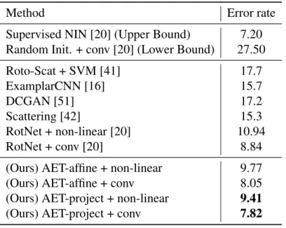
In Table 3.1, we compare the AET models with both fully supervised and unsupervised methods on CIFAR-10. First, we note that the unsupervised AET-project with the convolutional classifier almost achieves the same error rate as its fully supervised NIN counterpart with four convolutional blocks (7.82% vs. 7.2%). This is a remarkable result demonstrating AET is capable of training unsupervised features with a much narrower gap of performance to its supervised counterpart on CIFAR-10.

Table 3.1: Comparison between unsupervised feature learning methods on CIFAR-10.

Method Error rate

Supervised NIN [20] (Upper Bound) 7.20

Random Init. + conv [20] (Lower Bound) 27.50

Roto-Scat + SVM [41] 17.7 ExamplarCNN [16] 15.7 DCGAN [51] 17.2 Scattering [42] 15.3 RotNet + non-linear [20] 10.94 RotNet + conv [20] 8.84

(Ours) AET-affine + non-linear 9.77

(Ours) AET-affine + conv 8.05

(Ours) AET-project + non-linear 9.41

(Ours) AET-project + conv 7.82

(34)

Exam-plarCNN also applies various transformations to images, including rotations, translations, scaling and even more such as manipulating contrasts and colors. Then it trains unsupervised CNNs by classifying the resultant surrogate classes each containing all transformed versions of an individual images. Compared with ExamplarCNN [16], AET still has a significant lead in error rate, implying it can explore the image transformations more effectively in training unsupervised networks.

It is worth pointing out on CIFAR-10, the other reported methods [41, 16, 51, 42, 20] are usually based on different unsupervised networks and supervised classifiers for evaluation, making it dif-ficult to make a direct comparison between them. The results still suggest that the state-of-the-art performances can be reached by AETs, as their error rates are very close to the pre-assumptive lower bound set by the fully supervised counterpart.

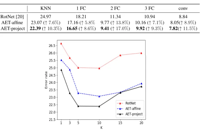
Indeed, one can choose the RotNet in Table 3.1 as the baseline for comparison as it is trained with the same network and classifier as the AETs. Thus we can make a fair comparison directly. From the results, AETs successfully beat the RotNet with both fully connected (FC) and convolutional classifiers on top of the learned representations. We also compare AETs with this baseline when they are trained with the KNN classifier and varying FC layers in Table 3.2. The results show that AET-project can consistently achieve the smallest errors no matter which classifiers are used. In Figure 3.3, we also compare the KNN results with varying number of nearest neighbors. Again, AET-project performs the best without involving any labeled examples. The model free KNN results suggest the AET model has an advantage when no labels are available in training classifiers upon the unsupervised features.

For the following ImageNet experiments, many existing methods have been compared in literature with the same unsupervised AlexNet architecture as well as the classifiers upon it for the evaluation. We will make a fair comparison directly, and the results show that AET still greatly outperforms the other unsupervised methods.

(35)

Table 3.2: Error rates of different classifiers on CIFAR 10.

KNN 1 FC 2 FC 3 FC conv

RotNet [20] 24.97 18.21 11.34 10.94 8.84

AET-affine 23.07 (↑7.6%) 17.16 (↑5.8% 9.77 (↑13.8%) 10.16 (↑7.1%) 8.05(↑8.9%) AET-project 22.39(↑10.3%) 16.65(↑ 8.6%) 9.41(↑17.0%) 9.92(↑9.3%) 7.82(↑ 11.5%)

Figure 3.3: The comparison of the KNN error rates by different models with varying numbers K of nearest neighbors on CIFAR-10.

3.2.2 ImageNet Experiments

We further evaluate the performance by AET on the ImageNet dataset. The AlexNet is used as the backbone to learn the unsupervised features. As shown by the results on CIFAR-10, the projective transformation has better performance on training the AET model, and thus we report the AET-project results here.

(36)

with original and transformed images as inputs respectively to train unsupervised AET-project. The4,096-d output features from the second last fully connected layer in two branches are con-catenated and fed into the output layer producing eight projective transformation parameters. We still use SGD to train the network, with a batch size of768 images and their corresponding trans-formed version, a momentum of0.9, a weight decay of5×10−4. The initial learning rate is set to

0.01, and it is dropped by a factor of10at epoch100 and150. AET is trained for200 epochs in total. Finally, the projective transformations applied are randomly sampled in the same fashion as on CIFAR-10.

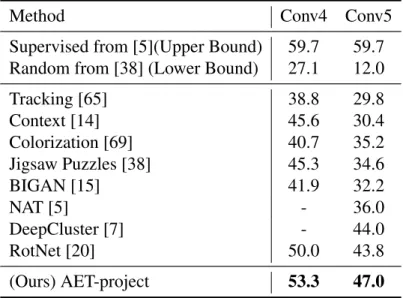
Results. First we report the Top-1 accuracies of compared methods in Table 3.3 on ImageNet by following the evaluation protocol in [38]. Two settings are adopted for evaluation – Conv4 and Conv5 denote to train the remaining part of AlexNet on top of Conv4 and Conv5 with the labeled data, while all the bottom convolutional layers up to Conv4 and Conv5 are frozen after they are trained in an unsupervised fashion. For example, in the Conv4 setting, Conv5 and three fully connected layers are trained on the labeled examples, including the last 1000-way output layer. From the results, in both settings, the AET model successfully beats the other compared unsupervised models. In particular, among the compared models is the BiGAN [15] that trains a GAN-based unsupervised model, and learns a databased auto-encoder as well to map an image to an unsupervised representation. Thus, it can be seen as combing the strengths of both GAN and AED models. The results show AET outperforms BiGAN by a significant lead, suggesting its advantage over the GAN and AED paradigms at least in this experiment setting.

We also compare with the fully supervised models that give the upper bounded performance by training the entire AlexNet with all labeled data. The classifiers of random models are trained on top of Conv4 and Conv5 with randomly sampled weights, and they set up the lower bounded performance. From the comparison, the AET models greatly narrow the performance gap to the upper bound – the gap to the upper bound Top-1 accuracy has been decreased from 9.7% and

(37)

15.7%by RotNet and DeepCluster on Conv4 and Conv5, respectively, to6.5%and12.7%by AET, which is relatively narrowed by33%and19%, respectively.

Table 3.3: ImageNet top-1 classification with non-linear layers

Method Conv4 Conv5

Supervised from [5](Upper Bound) 59.7 59.7

Random from [38] (Lower Bound) 27.1 12.0

Tracking [65] 38.8 29.8 Context [14] 45.6 30.4 Colorization [69] 40.7 35.2 Jigsaw Puzzles [38] 45.3 34.6 BIGAN [15] 41.9 32.2 NAT [5] - 36.0 DeepCluster [7] - 44.0 RotNet [20] 50.0 43.8 (Ours) AET-project 53.3 47.0

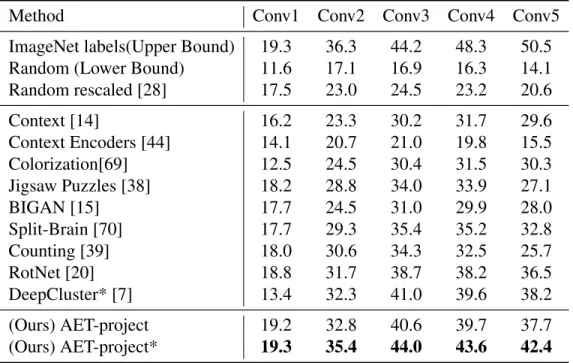
Moreover, we also follow the testing protocol adopted in [70] to compare the models by training a1,000-way linear classifier on top of different numbers of convolutional layers in Table 3.4. The models denoted with * where ten crops are applied to compare results. Again, AET obtains the best accuracy among all the compared unsupervised models.

3.2.3 Places Experiments

We also conduct experiments on the Places dataset. As shown in Table 3.5, we evaluate unsuper-vised models that are pretrained on the ImageNet dataset. Then a single-layer logistic regression classifier is trained on top of different layers of feature maps with Places labels. Thus, we assess the generalizability of unsupervised features from one dataset to another. Our models are still based on AlexNet variants like those used in the ImageNet experiments. We also compare with the

(38)

fully supervised models trained with the Places labels and ImageNet labels,as well as the random networks. The results show the AET models outperform the other unsupervised models in most of cases, except on Conv1 and Conv2, Counting [39] performs slightly better.

Table 3.4: ImageNet top-1 classification with linear layers.

Method Conv1 Conv2 Conv3 Conv4 Conv5

ImageNet labels(Upper Bound) 19.3 36.3 44.2 48.3 50.5

Random (Lower Bound) 11.6 17.1 16.9 16.3 14.1

Random rescaled [28] 17.5 23.0 24.5 23.2 20.6 Context [14] 16.2 23.3 30.2 31.7 29.6 Context Encoders [44] 14.1 20.7 21.0 19.8 15.5 Colorization[69] 12.5 24.5 30.4 31.5 30.3 Jigsaw Puzzles [38] 18.2 28.8 34.0 33.9 27.1 BIGAN [15] 17.7 24.5 31.0 29.9 28.0 Split-Brain [70] 17.7 29.3 35.4 35.2 32.8 Counting [39] 18.0 30.6 34.3 32.5 25.7 RotNet [20] 18.8 31.7 38.7 38.2 36.5 DeepCluster* [7] 13.4 32.3 41.0 39.6 38.2 (Ours) AET-project 19.2 32.8 40.6 39.7 37.7 (Ours) AET-project* 19.3 35.4 44.0 43.6 42.4

3.2.4 Analysis of Predicated Transformations

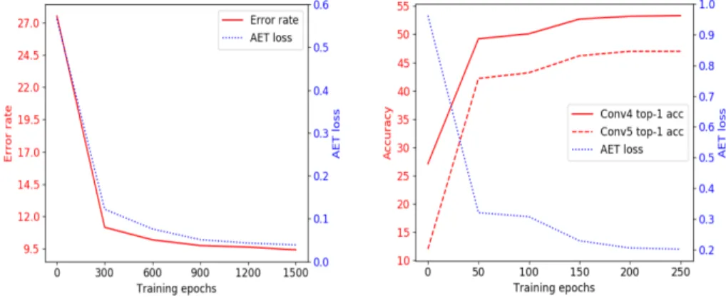
Although our ultimate goal is to learn good representations of images, it is insightful to look into the accuracy of predicting transformations and its relation with the supervised classification performance. As illustrated in Figure 3.4, the trend of transformation prediction loss (i.e. the AET loss being minimized to train the model) is well aligned with that of classification error and Top-1 accuracy on CIFAR-10 and ImageNet. This suggests that better prediction of transformations is a good surrogate of better classification result by using the learned features. This justifies our choice of AET to supervise the learning of feature representations.

(39)

Table 3.5: Places top-1 classification with linear layers.

Method Conv1 Conv2 Conv3 Conv4 Conv5

Places labels(Upper Bound)[71] 22.1 35.1 40.2 43.3 44.6

ImageNet labels 22.7 34.8 38.4 39.4 38.7

Random (Lower Bound) 15.7 20.3 19.8 19.1 17.5

Random rescaled [28] 21.4 26.2 27.1 26.1 24.0 Context [14] 19.7 26.7 31.9 32.7 30.9 Context Encoders [44] 18.2 23.2 23.4 21.9 18.4 Colorization[69] 16.0 25.7 29.6 30.3 29.7 Jigsaw Puzzles [38] 23.0 31.9 35.0 34.2 29.3 BIGAN [15] 22.0 28.7 31.8 31.3 29.7 Split-Brain [70] 21.3 30.7 34.0 34.1 32.5 Counting [39] 23.3 33.9 36.3 34.7 29.6 RotNet [20] 21.5 31.0 35.1 34.6 33.7 DeepCluster* [7] 19.6 33.2 39.2 39.8 34.7 (Ours) AET-project 22.1 32.9 37.1 36.2 34.7 (Ours) AET-project* 23.0 34.4 39.0 38.4 37.4

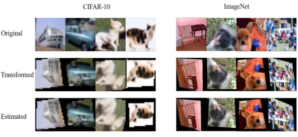
In Figure 3.5, we also compare some examples of original images, along with the transformed im-ages at the input and the output ends of the AET model. These examples show how well the model can decode the transformations from the encoded image features, thereby delivering unsupervised representations that offer competitive performances on classifying images in our experiments.

Figure 3.4: Error rate (top-1 accuracy) vs. AET loss over epochs on the CIFAR-10 and ImageNet datasets.

(40)

(41)

CHAPTER 4: INVARIANCE AGAINST PERTURBATIONS ON DATA

MANIFOLD

In this chapter, we start to discuss the critical roles played by the invariance against perturbations for stable and smooth predictions. We present a novel Localized Generative Adversarial Networks (LGAN) [49] to directly learn and access to the local data manifold. It addresses the problem of non-existence of global coordinate and local mode collapse with the locality and orthonormality natures. To train a locally consistent classifier invariant against perturbations on the manifold, we will show the superior performances of LGAN on the semi-supervised learning application.

The classic Generative Adversarial Net (GAN) [22] seeks to generate samples with indistinguish-able distributions from real data. For this purpose, it learns a generatorG(z)as a function that maps from input random noiseszdrawn from a distributionPZ to output dataG(z). A discriminator is

learned to distinguish between real and generated samples. The generator and discriminator are jointly trained in an adversarial fashion so that the generator fools the discriminator by improving the quality of generated data.

All the samples produced by the learned generator form a manifoldM = {G(z)|z ∼ PZ}, with

the input variables z as its global coordinates. However, a global coordinate system could be too restrictive to capture various forms of local transformations on the manifold. For example, a nonrigid object like human body and a rigid object like a car admit different forms of variations on their shapes and appearances, resulting in distinct geometric structures unfit into a single coordinate chart of image transformations.

Indeed, existence of a global coordinate system is a too strong assumption for many manifolds. For example, there does not exist a global coordinate chart covering an entire hyper-sphere embedded

(42)

in a high dimensional space as it is even not topologically similar (i.e., homeomorphic) to an Euclidean space. This prohibits the existence of a global isomorphism between a single coordinate space and the hyper-sphere, making it impossible to study the underlying geometry in a global coordinate system. For this reason, mathematicians instead use an atlas of local coordinate charts located at different points on a manifold to study the underlying geometry [19].

Even when a global coordinate chart exists, a global GAN could still suffer two serious challenges. First, a pointxon manifold cannot be directly mapped back to its global coordinatesz, i.e., finding

z such as G(z) = x for a givenx. But many applications need the coordinates of a given point

x to access its local geometry such as tangents and curvatures. Thus, for a global GAN, one has to solve the inverse G−1 of a generator network (e.g., via an autoencoder such as VAE [26], ALI [17] and BiGAN [15]) to access the coordinates of a point x and then its local geometry of data transformations along the manifold.

The other problem is the manifold generated by a global GAN could locally collapse. Geometri-cally, on a N-dimensional manifold, this occurs if the tangent spaceTxof a pointxis dimensionally

deficient, i.e., dimTx < N when tangents become linearly dependent along some coordinates . In

this case, data variations become redundant or even vanish along some directions on the mani-fold. Moreover, a locally collapsed tangent space at a point x could be related with a collapsed mode[22, 56], around which a generatorG(z)would no longer produce diverse data as zchanges in different directions. This provides us with an alternative geometric insight into mode collapse phenomena observed in literature [51].

The above challenges inspire us to develop a Localized GAN (LGAN) by learning local generators

G(x, z)associated with individual pointsxon a manifold. As illustrated in Figure 1, local genera-tors are located around different data points so that the pieces of data generated by different local generators can be sewed together to cover an entire manifold seamlessly. Different pieces of

(43)

gen-erated data are not isolated but could have some overlaps between each other to form a connected manifold [47].

Figure 4.1: Illustration of a curved manifoldMembedded in3- dimensional ambient space.

The advantage of the LGAN is at least twofold. First, one can directly access the local geometry of transformations near a point without having to evaluate its global coordinates, as each point is directly localized by a local generator in the corresponding local coordinate chart. This locality nature of LGAN makes it straightforward to explore pointwise geometric properties across a man-ifold. Moreover, we will impose an orthonormality prior on the local tangents, and the resultant orthonormal basis spans a full dimensional tangent space, preventing a manifold from being locally collapsed. It allows the model to explore diverse patterns of data transformations disentangled in different directions, leading to a geometric approach at least locally alleviating the mode collapse problem on a manifold.

We will also demonstrate an application of the LGAN to train a robust classifier invariant against perturbations by encouraging a smooth change of the classification decision on the manifold formed by the LGAN. The classifier is trained with a regularizer that minimizes the square norm of the classifier’s gradient on the manifold, which is closely related with Laplace-Beltrami operator.

(44)

The local coordinate representation in LGAN makes it straightforward to train such a classifier with no need of computing global coordinates of training examples to access their local geome-try of transformations. Moreover, the learned orthonormal tangent basis also allows the model to effectively explore various forms of independent transformations allowed on the underlying mani-fold.

4.1 Localized GANs

We present the proposed Localized GANs (LGANs). Before that, we first briefly review the classic GANs in the context of differentiable manifolds.

4.1.1 Classic GAN and Global Coordinates

A Generative Adversarial Net (GAN) seeks to train a generatorG(z) by transforming a random noise z ∈ _RN _{drawn from} _P

Z to a data sampleG(z) ∈ RD. Such a classic GAN uses a global

N-dimensional coordinate systemzto represent its generated samplesG(z)residing in an ambient spaceRD. Then all the generated samples form a N-dimensional manifoldM={G(z)|z ∈RN}

that is embedded in_RD_.

In a global coordinate system, the local structure (e.g., tangent vectors and space) of a given data point x is not directly accessible, since one has to compute its corresponding coordinates z to localize the point on the manifold. One often has to resort to an inverse of the generator (e.g., via ALI and BiGAN) to find the mapping fromxback toz.

Even worse, the tangent spaceTxcould locally collapse at a pointxif it is dimensionally deficient

(45)

xcould become a collapsed mode on the manifold, around whichG(z)would no longer produce significant data variations even though z changes in different directions. For example, if dim Tx = 1, there is only a curve of data variations passing throughx. In an extreme case dimTx = 1,

the data variations would completely vanish asxbecomes a singular point on the manifold.

4.1.2 Local Generators and Tangent Spaces

Unlike the classic GAN, we propose a Localized GAN (LGAN) model equipped with a local generatorG(x, z)that can produce various examples in the neighborhood of a pointx ∈ _RD _on

the manifold.

This forms a local coordinate chart{G(x, z)|z ⊂ _RN _∼ _P

Z}aroundx, with its local coordinates

z drawn from a random distribution PZ over an Euclidean spaceRN. In this manner, an atlas of

local coordinate charts can cover an entire manifoldMby a collection of local generatorsG(x, z)

located at different points onM.

In particular, forG(x, z), we assume that the origin of the local coordinates z should be located at the given pointx, i.e.,G(x,0) =x, where0∈_RN _{is an all-zero vector.}

To study the local geometry near a pointx, we need tangent vectors located atxon the manifold. By changing the value of a coordinatezj _{while fixing the others, the points generated by}_G₍_{x, z}₎

form a coordinate curve passing through x on the manifold. Then, the vector tangent to this coordinate curve atxis

τ_xj=4 ∂G(x, z)

∂zj |z=0 ∈R D

(4.1)

All suchN tangent vectorsτj

x,j = 1, ..., N form a basis spanning a linear tangent spaceTx=Span (τ1

(46)

xon the manifold. Each tangent τ ∈ Tx characterizes some local transformation in the direction

of this tangent vector.

A Jacobian matrix Jx ∈ RD×N can also be defined by stacking all N tangent vectors τxj in its

columns.

4.1.3 Regularity: Locality and Orthonormality

However, there exists a challenge that the tangent spaceTx would collapse if it is dimensionally

deficient, i.e, its dimension dimTx is smaller than the manifold dimension N. If this occurs, the

N tangents in 4.1 could reduce to dependent transformations that would even vanish along some coordinatesz.

To prevent the collapse of the tangent space, we need to impose a regularity condition that theN

basis{τ_xj, j = 1, ..., N} ofTx should be linearly independent of each other. This guarantees the

manifold be locally “similar” (diffeomorphic mathematically) to a N-dimensional Euclidean space, rather than being collapsed to a lowerdimensional subspace having dependent local coordinates.

As a linearly independent basis can always be transformed to an orthonormal counterpart by a proper transformation, one can set the orthonormal condition on the tangent vectorsτj

x, i.e.,

< τ_xi, τ_xj >=δij (4.2)

whereδij = 0fori 6=j andδij = 1otherwise. The resultant orthonormal basis of tangent vectors

capture the independent components of local transformations near individual data points on the manifold.

(47)

(i) locality: G(x,0) = x, i.e., the origin of the local coordinateszshould be located atx;

(ii) orthonormality:JT_xJx =IN, which is a matrix form of 4.2 withIN being the identity matrix of

sizeN.

One can minimize the following regularizer onG(x, z)to penalize the violation of these two con-ditions,

ΩG(x) =µ||G(x,0)−x||2+η||JTxJx−IN||2 (4.3)

whereµandηare nonnegative weighting coefficients for the two terms. By using a deep network for computingG(x, z), this regularizer can be minimized by backpropagation algorithm.

4.1.4 Training G(x,z)

Now the learning problem for the localized GANs boils down to train aG(x, z). Like the GANs, we will train a discriminatorD(x)to distinguish between real samples drawn from a data distribution

PX and generated samples byG(x, z)withx∼PX andz ∼PZ as follows.

max

D Ex∼PXlog(D(x)) +Ex∼PX,z∼PZlog(1−D(G(x, z)))

whereD(x)is the probability of xbeing real, and the maximization is performed wrt the model parameters of discriminatorD.

On the other hand, the generator can be trained by maximizing the likelihood that the generated samples byG(x, z)are real as well as minimizing the regularization term 4.3.

min

G −Ex∼PX,z∼PZlogD(G(x, z)) +Ex∼PXΩG(x)

(48)

regularization enforces the locality and orthonormality conditions onG.

ThenDandGcan be alternately optimized by stochastic gradient descent via a backpropagation algorithm.

4.2 Semi-Supervised LGANs

In this section, we will show that the LGAN can help us train a locally consistent classifier by exploring the manifold geometry. First we will discuss the functional gradient on a manifold in Section 4.2.1, and show its connection with Laplace-Beltrami operator that generalizes the graph Laplacian in Section 4.2.2. Finally, we will present the proposed LGAN-based classifier in detail in Section 4.2.3.

4.2.1 Functional Gradient along Manifold

First let us discuss how to calculate the derive of a function on the manifold.

Consider a function f(x) defined on the manifold. At a given point x, its neighborhood on the manifold is depicted byG(x, z)with the local coordinatesz. By viewingf as a function ofz, we can compute the derivative off when it is restricted on the manifold.

It is not hard to obtain the derivative of f(G(x, z)) with respect to a coordinatezj by the chain rule,

∂f(G(x, z))

∂zj |z=0 =< τ j

x,5xf(x)>

where5xf(x)is the gradient off atx, and<·,· >is the inner product between two vectors. It

(49)

Then, the gradient off atxwhenf is restricted on the manifoldG(x, z)can be written as

5G_xf _,5zf(G(x, z))|z=0 =JxT 5xf(x) (4.4)

Geometrically, it shows the gradient of f along the manifold can be obtained by projecting the regular gradient5xf onto the tangent spaceTxwith the Jacobian matrixJx. Here we denote the

resultant gradient along manifold by5G

xf to highlight its dependency onG(x, z)

4.2.2 Connection with Laplace-Beltrami Operator

Iff is a classifier,5zf(G(x, z))depicts the change of the classification decision on the manifold

formed byG(x, z). Atx, the change off restricted onG(x, z)can be written as

|f(G(x, z+δz))−f(G(x, z))|2 _{≈ || 5}G x f||

2_δz

(4.5)

It shows that penalizing || 5G

x f||2 can train a robust classifier that is resilient against a small

perturbationδzon a manifold. It is supposed to deliver locally consistent classification results in presence of noises.

The functional gradient is closely related with the Laplace-Beltrami operator, the one that is widely used as a regularizer on the graph-based semi-supervised learning [3, 4, 74, 73].

It is well known that the divergence operator div and the gradient5are formally adjoint, i.e.,R_M <

V,5G

xf > dPX = R

Mdiv(V)f dPX. Thus we have

Z M || 5G x f|| 2_dP X = Z M f div(5G xf)dPX (4.6) where4f _,div(5G

(50)

In graph-based semi-supervised learning, one constructs a graph representation of data points to approximate the underlying data manifold [4], and then use a Laplacian matrix to approximate the Laplace-Beltrami operator4f.

In contrast, with the help of LGAN, we can directly obtain4fonG(x, z)without having to resort to a graph representation. Actually, as the tangent space at a pointxhas an orthonormal basis, we can write 4f =div(5G xf) = N X j=1 ∂2_f₍_G₍_{x, z}₎₎ ∂(zi₎2 (4.7)

In the following, we will learn a locally consistent classifier on the manifold by penalizing a sudden change of its classification function f in the neighborhood of a point. We can implement it by minimizing either the square norm of the gradient or the related Laplace-Beltrami operator. For simplicity, we will choose to penalize the gradient of the classifier as it only involves computing the firstorder derivatives of a function compared with the Laplace-Beltrami operator having the higher-order derivatives.

4.2.3 Locally Consistent Semi-Supervised Classifier

We consider a semi-supervised learning problem with a set of training examples (xl, yl) drawn

from a distributionPLof labeled data. We also have some unlabeled examplesxudrawn from the

data distributionPX of real samples. The amount of unlabeled examples is often much larger than

their labeled counterparts, and thus can provide useful information for training G to capture the manifold structure of real data.

Suppose that there areKclasses, and we attempt to train a classifierP(y|x)fory∈ {1,2, ..., K+ 1}that outputs the probability of xbeing assigned to a class y[56]. The first K are real classes and the last one is a fake class denotingxis a generated example.

(51)

This probabilistic classifier can be trained by the following objective function max P E(xl,yl)∼PLlogP(yl|xl) +Exu∼PXlogP(yu ≤K|xu) +_Ex∼PX,z∼PZlogP(y=K+ 1|G(x, z)) − K X k=1 Ex PX|| 5 G x logP(y=k|x)|| 2 (4.8)

where of the last term5G

xlogP(y =k|x)is the gradient of the log-likelihood along the manifold

G(x, z)atx, that is5zogP(y=k|G(x, z))|z=0. Let us explain the objective4.8 in detail below.

• The first term maximizes the log-likelihood that a labeled training example drawn from the distributionPLof labeled examples is correctly classified byP(y|x).

• The second term maximizes the log-likelihood that an unlabeled examplexu drawn from the

data distributionPX is assigned to one ofK real classes (i.e.,yu ≤K).

• The third term enforcesP(y|x)to classify a generated sample byG(x, z)as fake (i.e.,y =

K+ 1).

• The last term penalizes a sudden change of classification function on the manifold, thus yielding a locally consistent classifier as expected. This can be seen by viewinglogP(y|x)

asf in 4.5.

On the other hand, with a fixed classifierP(y|x), the local generatorGis trained by the following objective:

min

G KG+LG+Ex∼PXΩG(x) (4.9)

(52)

• The first term is label preservation term KG = −E(xl,yl)∼PL,z∼P_ZlogP(yl|G(xl, z)) which enforces generated samples should not change the labels of their original examples. This label preservation term can help explore intra-class variance by generating new variants of training examples without changing their labels.

• The second term is feature matching lossLG =||Ex∼PXϕP(x)−Ex∼PX,z∼PZϕP(G(x, z))||

2

, whereϕP is an intermediate layer of feature representation from the classification network

P. It minimizes the feature discrepancy between real and generated examples, and exhibits competitive performance in literature [56, 31] for semi-supervised learning.

• The third term is the regularizerΩG(x)that enforces the locality and orthonormality priors

on the local generator as shown in 4.3.

4.3 Experiments

In this section, we conduct experiments to test the capability of the proposed LGAN on both image generation and classification tasks.

4.3.1 Architecture and Training Details

In this section, we discuss the network architecture and training details for the proposed LGAN model in image generation and claudication tasks.

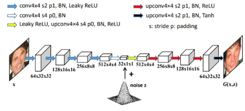
In experiments, the local generator networkG(x, z)was constructed by first using a CNN to map the input image x to a feature vector added with a noise vector of the same dimension. Then a deconvolutional network with fractional strides was used to generate output imageG(x, z). Fig-ure 4.2 illustrates the architectFig-ure for the local generator network used to produce images on

(53)

CelebA. The same discriminator network as in DCGAN[51] was used in LGAN. The detail of network architectures used in semi-supervised classification tasks will be discussed shortly.

Figure 4.2: Network architecture for local generators on the CelebA dataset.

Instead of drawingzfrom a Gaussian distribution, the quality of generated images can be improved by training the LGAN with noises sampled from a mixture of Gaussian noise with a discrete distributionδ0concentrated at 0, i.e.,z ∼0.9N(0, I) + 0.1δ0whereN(0, I)is zero-mean Gaussian distribution with an identity covariance matrixI. In other words, with a probability of0.1,z is set to0; otherwise, with probability of0.9, it is drawn fromN(0, I). Sampling fromδ0 could better serve to enforce the locality prior when training a local generator in its local coordinate chart.

We used Adam solver to update the network parameters where the learning rate is set to5×10−5 and10−3 _{for training discriminator and generator networks respectively. The two hyperparameters}

µand η imposing locality and orthonormality priors in the regularizer were chosen based on an independent validation set held out from the training set.