Spam Detection Using Machine Learning

33

Spam Detection Using Machine Learning

Department of Electrical Engineering, Louisiana State University Patrick F. Taylor Hall, Baton Rouge, LA 70808

Abstract

Emails are essential in present century communication however spam emails have contributed negatively to the success of such communication. Studies have been conducted to classify messages in an effort to distinguish between ham and spam email by building an efficient and sensitive classification model with high accuracy and low false positive rate. Regular rule-based classifiers have been overwhelmed and less effective by the geometric growth in spam messages, hence the need to develop a more reliable and robust model. Classification methods employed includes SVM (support vector machine), Bayesian, Naïve Bayes, Bayesian with Adaboost, Naïve Bayes with Adaboost. However, for this project, the Bayesian was employed using Python programming language to develop a classification model.

Keywords: machine learning (ML), machine learning classifier, Naïve Bayes, SVM, Adaboost, spam classification, ham.

DOI: 10.7176/CEIS/11-3-04 Publication date:May 31st ₂₀₂₀

1. Introduction

In recent years, there has been an increase in unsolicited commercial / bulk e-mail also called spam, which has become a big trouble over the internet. Spam message wastes storage space, time, as well as bandwidth. This problem has been on the increase for years. In recent statistics, 45% of all emails are spam which about 15.6 billion email per day and that cost internet users over $300 million per year. An automatic e-mail filtering appears to be the most effective method to counter spam at the moment. With improving trickery from spammers, the classic solution of blocking a certain email address or filtering messages with certain subject lines have not been effective. Use of random sender addresses and/or append random characters to the beginning or the end of the message subject line by the spammers have effectively negated the classic approach. Knowledge engineering and machine learning are the two general approaches used in e-mail filtering. The use of a set of rules specified to which emails are categorized as spam or ham is referred to as knowledge engineering. This set of rules should be created either by the user of the filter, or by some other authority (e.g. the software company). Figure 1 shows a typical email spam deployment process. This method is effective to a specific set of messages defined as spam; hence it must be constantly updated and maintained to keep up with ever increasing type of spam messages. This is a waste of time and it is not convenient for most users. Machine learning has often been viewed in the same vein as rocket science when reported.

Fig 1 Typical spam filter

However, in reality, it is quite simpler than it poses. Machine learning refers to the ability of computers to learn to do something, without the need to explicitly program them for the task. Machine learning approach is

34

more efficient than knowledge engineering approach, as it does not require specifying any rules. Instead, a set of training samples, these samples is a set of pre-classified e-mail messages, is used to train an algorithm which is then set to classify in coming emails. Machine learning system is trained rather than explicitly programmed, data is inputted as well as the answers expected from the data and out comes the rules. Once the rules have been obtained, the system is said to have been trained. A way to measure whether the algorithm is doing a good job is to have a feedback to show how close the prediction is to the actual value. The adjustment step is called learning. First, the algorithm is made to look at a certain set of data, in order to train it for the task. Then, we give the algorithm data it has never seen before and perform the task on this data. A specific algorithm is then used to learn the classification rules from these e-mail messages. Machine learning approach has been widely studied and there are lots of algorithms can be used in e-mail filtering. They include Naïve Bayes, K-nearest neighbor, Neural Networks, support vector machines and the artificial immune system. Deep learning is a section of subfield of machine learning, it stands for the idea of successive layers of data representation which are learned habitually from introduction to training data set. A deep network can be thought of as information-distillation operation, where information goes through successive filters and comes out increasingly purified. Modern deep learning often has tens or even hundreds of successive layers of representation. This paper considered Naïve Bayes neural network system, implemented using python programming language on Jupyter notebook.

2Structure of a usual Spam filter

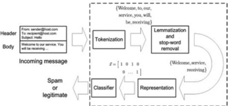
The information contained in the email message is divided into the header; this field includes general information on the message, such as the subject, sender and recipient, the body; the actual contents of the message. Prior to classification of the message into spam or ham by a classifier, the message must be first filtered. This involves, extraction of the words in the message body (tokenization), reducing them to their root forms, eliminate some words that are usually used in many messages (stop words) and the presentation the set of words in a specific format to the algorithm. Fig 1 shows this process.

Fig 2 Illustration of steps involved in a spam filter.

A classifier is a function f that maps input feature vectors x ∈ X to output class labels y ∈ {1, . . . , C}, where X is the feature space. We will typically assume ꭓ = RD _{or ꭓ = {0, 1}} D_{, i.e., that the feature vector is a vector}

of D real numbers or D binary bits, but in general, we may mix discrete and continuous features. The goal is to learn f from a labeled training set of N input-output pairs, i.e. supervised learning.

A simple illustration is; Input: X = email messages

Header: From: Date: Subject: Body:

Output: y ∈ {spam, not spam}

Hence the objective is to obtain a predictor f that maps an input x to output y.

In deep learning the system does not need the data to be pre-processed; it learns the feature directly from the data set. It is also able to handle higher amount of data compare to machine learning producing a better performance. For this project two set of data was used, one for machine learning and the other for deep learning.

3.1 Naïve Bayes Classifier

This is a method of classification based on Bayes theorem. The conditional probability of an event is a probability obtained with the additional information that some other event has already occurred. P(B|A) is used to denote the conditional probability of event B occurring, given that event A has already occurred. The following formula was provided to obtain P(B|A):

35

(1)

A prior probability is an initial probability value originally obtained before any additional information is obtained. A posterior probability is a probability value that has been revised by using additional information that is later obtained.

Bayes' Theorem

The probability of event A, given that event B has subsequently occurred, is

(2)

Where A and B are events and P(B) ≠ 0.

P(A|B) is a conditional probability: the likelihood of event A occurring given B is true. P(B|A) is also a conditional probability, the likelihood of event B occurring given A is true. The Naïve Bayes classifier calculates the probabilities for every factor. Then it selects the outcome with highest probability.

(3)

(4) For the purpose of this research, rewriting the Naïve Bayes equation gives:

What we want is: P (spam | words)

(5)

Assume independence: probability of each word independent of others

| 1| 2| . . . |

3.2 AdaBoost

The term ‘Boosting’ refers to a family of algorithms which converts weak learner to strong learners. Boosting is an approach to machine learning based on the idea of creating a highly accurate prediction rule by combining many relatively weak and inaccurate rules. Adaptive boosting works to re-weight the data rather random sampling. This method develops a concept of building ensembles for performance improvement of the classifiers. AdaBoost (Adaptive boosting) classifier builds a strong classifier by combining multiple poorly performing classifiers so that you will get high accuracy strong classifier. The basic concept behind Adaboost is to set the weights of classifiers and training the data sample in each iteration such that it ensures the accurate predictions of unusual observations. Any machine learning algorithm can be used as base classifier if it accepts weights on the training set. Adaboost should meet two conditions:

1. The classifier should be trained interactively on various weighed training examples.

2. In each iteration, it tries to provide an excellent fit for these examples by minimizing training error. The goal of boosting is to improve the accuracy of any given learning algorithm.

AdaBoost is popular for a number of reasons: • It has no tricky parameters to set.

• It is computationally tractable and not too hard to implement. • It generalizes very well and avoids overfitting.

• It satisfies some nice theoretical guarantees, as we will see later in this lecture and next time.

Weak Learner: A simple rule-of-the-thumb classifier that doesn’t necessarily work very well. A class of concepts is learnable (or strongly learnable) if there exists a polynomial-time algorithm that achieves low error with high confidence for all concepts in the class. A weaker model of learnability, called weak learnability, drops the requirement that the learner be able to achieve arbitrarily high accuracy; a weak learning algorithm need only output an hypothesis that performs slightly better (by an inverse polynomial) than random guessing. Let D be a distribution over examples, and h be a classifier Error of h with respect to D is:

ErrorD (h(x)) ≡ Pr (X,Y )∼D(h(X) ≠ Y ) h is called a weak learner if ErrorD (h(x))< 0.5

With Adaboost, instead of sampling uses training set re-weighting each training sample uses a weight to determine the probability of being selected for a training set.

)

(

)

(

)

|

(

)

|

(

words

P

spam

P

spam

words

P

words

spam

P



(words P words spam P spam P words good P good

36

– Previous weak learner has only 50% accuracy over new distribution – Can be used to learn weak classifiers

– Final classification based on weighted vote of weak classifiers

Fig 3 Structure of an adaptive filter

ℎ

(6)

The selected weight for each new weak classifier is always positive. The smaller the classification error, the bigger the weight and the more this particular weak classifier will impact the final strong classifier.

Ɛ(ha) < Ɛ(hb) >

(7) Weight of classifier is straight forward; it is based on the error rate Ɛ. Ɛ is just the number of misclassifications over the training set divided by the training set size. After weak classifier is trained, we update the weight of each training example with following

_!" (i) = #$% &'( )*_/ $+$,$-.

$ (8)

We normalize the weights by dividing each of them by the sum of all the weights, Zt. 3.3 Support Vector Machine

Support vector model (SVM) seeks to draw a hyperplane to classify points in a finite dimensional space. SVM is a supervised learning model, i.e. it requires labeled input and output data or pattern be fed into the system, used for classification and regression analysis. For this paper linear SVM classifier is used, however it can efficiently accomplish a non-linear classification by employing the kernel trick. Given two classes,

yi∈ {-1, 1} and there are n training samples, (x1, y1), ……, (xn, yn). if we run with the assumption that these two

classes are linearly separable, then an optimal weight vector w can be obtained. A linear classifier is explained using the diagram below:

f(x) = w

T

37

From the diagram above the support vector classifier (SVC), drew an optimal hyperplane to separate the two points and introduce a maximum margin.

w T . x + b < 0 predicts +1 w T . x + b = 0 On the hyperplane w T . x + b > 0 predicts -1 Mathematically the margin is maximized at 2/|W|.

4. Machine Learning

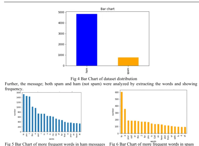
In this section, the dataset used was SMS Spam Collection of tagged messages that have been collected for SMS Spam research. It contained one set of SMS messages in English of 5,574 messages, tagged according being ham (legitimate) or spam. The files contain one message per line. Each line is composed by two columns: v1 contains the label (ham or spam) and v2 contains the raw text. NumPy library; fundamental package for scientific computing with Python, was used for the analysis. Pandas was used for loading the dataset unto the program.

38

Fig 4 Bar Chart of dataset distribution

Further, the message; both spam and ham (not spam) were analyzed by extracting the words and showing its frequency.

Fig 5 Bar Chart of more frequent words in ham messages Fig 6 Bar Chart of more frequent words in spam Text preprocessing, tokenizing and filtering of stop words are included in a high-level component that can build a dictionary of features and transform documents to feature vectors. For better analysis, the stop words were removed. The two possible outcome is either to predict spam as ham (false negative) or ham as spam (false positive). However, having a false positive is worse in this case because the ham message goes into spam and the recipient does not read it. The feature vector was converted to binary (spam = 1 and ham = 0) and split into training set and the testing set. The data set was applied using a regularization parameter α.

5. Result

In this section all the results obtained from the experiment was compiled and observed analytically. Obtaining a result of correct classification is the main goal, however the most important basis to determine the most effective of the methods is based on the ability of the model to accurately predict a ham message (precision).

5.1Naïve Bayes

Table 1. Table showing result using multi-nominal Naïve Bayes with varying alpha

It was observed that a test precision of 1.0 was obtained when the hyperparameter, alpha, was 15.73. The model produced a perfect classification of ham messages while wrongly classifying 62 spam messages.

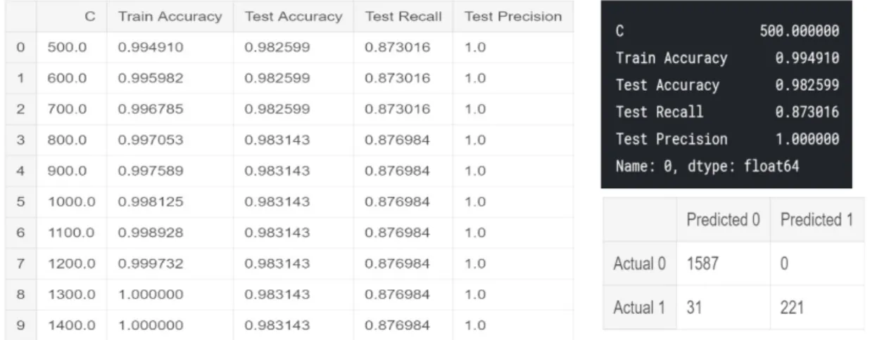
39 5.2 Support Vector Classifier

Table 2. Table showing result using the SVC with varying C

C is the regularization parameter. It determines the size of the margin. For large value of C, the hyperplane margin is small to ensure that all or most of the training points are classified correctly. However, for small value of C, the optimizer finds a hyperplane with a large margin at the cost of misclassifying some points. Hence adjusting the C parameter is a trade-off between obtaining low training error and low testing error. From the table above, the accurate with a small C was obtained when C was set to 500. SVC like Naïve Bayes produced a result that correctly classifies all the ham messages while wrongly classifying 31 spam messages. In other words, it has a high lower negative relative to the Naïve Bayes.

5.3 AdaBoost

The AdaBooost model was employed using SVC as the base classifier. Table 3. Using a learning rate of 0.5 with different weak classifiers

Number of weak classifiers Base Estimator Learning rate Test Accuracy

50 SVC 0.5 0.9821

100 SVC 0.5 0.9810

150 SVC 0.5 0.9766

Table 4. Using a learning rate of 0.25 with different weak classifiers

Number of weak classifiers Base Estimator Learning rate Test Accuracy

50 SVC 0.25 0.9864

100 SVC 0.25 0.9858

150 SVC 0.25 0.9858

Table 5. Using a learning rate of 0.1 with different weak classifiers

Number of weak classifiers Base Estimator Learning rate Test Accuracy

50 SVC 0.1 0.9858

100 SVC 0.1 0.9858

40

Table 6. Using 150 weak classifiers and 0.3 learning rate.

From the tables above, it is seen that getting a balance between the learning rate and base classifier affects the test accuracy and precision. The best value was obtained using 150 weak classifiers with learning rate of 0.3. It also wrongly classifies one ham message and 26 spam messages.

6. Conclusion

From the obtained results, it can be deduced that the native Bayes classification is 100% efficient as some spam messages were misclassified. SVC also produced no false positives with less false positives compared to Naïve Bayes. Finally, the use of number of combined SVC classifiers in and Adaboost model produce a more balanced result. It misclassified one spam message however with less misclassification of spam as ham. Future research in this area can be geared towards developing a deep learning model that can offer a better classification rate. References

Awad, W. (2011). Machine Learning Methods for Spam E-Mail Classification. International Journal of Computer Science and Information Technology, 3(1), 173-184. doi:10.5121/ijcsit.2011.3112

C. Ross Quinlin, C4.5: Programs for Machine Learning. San Mateo, CA: Morgan Kaufmann, 1988.

Deep Learning Tutorial for Beginners | Kaggle. (n.d.). Retrieved from https://www.kaggle.com/kanncaa1/deep-learning-tutorial-for-beginners/notebook

Guzella, T. S., & Caminhas, W. M. (2009). A review of machine learning approaches to Spam filtering. Expert Systems with Applications, 36(7), 10206-10222. doi:10.1016/j.eswa.2009.02.037

Larsen, K. (2005). Generalized Naive Bayes Classifiers. ACM SIGKDD Explorations Newsletter, 7(1), 76-81. doi:10.1145/1089815.1089826

Naive Bayes & SVM Spam Filtering | Kaggle. (n.d.). Retrieved from https://www.kaggle.com/pablovargas/naive-bayes-svm-spam-filtering/notebook

41 European Conf. Machine Learning, 1998.

Trivedi, S. K. (2016). A study of machine learning classifiers for spam detection. 2016 4th International Symposium on Computational and Business Intelligence (ISCBI). doi:10.1109/iscbi.2016.7743279

Visani, C., Jadeja, N., & Modi, M. (2017). A study on different machine learning techniques for spam review detection. 2017 International Conference on Energy, Communication, Data Analytics and Soft Computing (ICECDS). doi:10.1109/icecds.2017.8389522

[Wang and Manning2012] Sida Wang and Christopher D Manning. 2012. Baselines and bigrams: Simple, good sentiment and topic classification. In ACL.

[Weinberger et al.2009] Kilian Weinberger, Anirban Dasgupta, John Langford, Alex Smola, and Josh Attenberg. 2009. Feature hashing for large scale multitask learning. In ICML.

[Weston et al.2011] Jason Weston, Samy Bengio, and Nicolas Usunier. 2011. Wsabie: Scaling up to large vocabulary image annotation. In IJCAI.

[Weston et al.2014] Jason Weston, Sumit Chopra, and Keith Adams. 2014. #tagspace: Semantic embeddings from hashtags. In EMNLP.

[Xiao and Cho2016] Yijun Xiao and Kyunghyun Cho. 2016. Efficient character-level document classification by combining convolution and recurrent layers. arXiv preprint arXiv:1602.00367.

[Zhang and LeCun2015] Xiang Zhang and Yann LeCun. 2015. Text understanding fromscratch. arXiv preprint arXiv:1502.01710.

[Zhang et al.2015] Xiang Zhang, Junbo Zhao, and Yann LeCun. 2015. Character-level convolutional networks for text classification. In NIPS