University of Nebraska - Lincoln University of Nebraska - Lincoln
DigitalCommons@University of Nebraska - Lincoln
DigitalCommons@University of Nebraska - Lincoln
Dissertations and Theses in Agricultural
Economics Agricultural Economics Department
Summer 8-2011
Applying Data Mining Techniques to Evaluate Applications for
Applying Data Mining Techniques to Evaluate Applications for
Agricultural Loans
Agricultural Loans
Emile Salame
University of Nebraska-Lincoln, [email protected]
Follow this and additional works at: https://digitalcommons.unl.edu/agecondiss Part of the Agricultural and Resource Economics Commons
Salame, Emile, "Applying Data Mining Techniques to Evaluate Applications for Agricultural Loans" (2011). Dissertations and Theses in Agricultural Economics. 10.
https://digitalcommons.unl.edu/agecondiss/10
This Article is brought to you for free and open access by the Agricultural Economics Department at
DigitalCommons@University of Nebraska - Lincoln. It has been accepted for inclusion in Dissertations and Theses in Agricultural Economics by an authorized administrator of DigitalCommons@University of Nebraska - Lincoln.
APPLYING DATA MINING TECHNIQUES TO EVALUATE APPLICATIONS FOR AGRICULTURAL LOANS
by
Emile J. Salame
A DISSERTATION
Presented to the Faculty of
The Graduate College at the University of Nebraska
In partial Fulfillment of Requirements
For the Degree of Doctor of Philosophy
Major: Agricultural Economics
Under the Supervision of Professor Dennis M. Conley
Lincoln, Nebraska
APPLYING DATA MINING TECHNIQUES TO EVALUATE
APPLICATIONS FOR AGRICULTURAL LOANS
Emile J. Salame, Ph.D.
University of Nebraska, 2011
Adviser: Dennis M. Conley
Abstract
Financial lending institutions continuously look at improving their credit risk models. This study examines the performance of three estimation methods: logistic regression, decision tree, and neural networks, in terms of their misclassification rates of credit default. The study uses 17,328 loans of grain producers for the period of 2006 - 2010.
Those loans belong to the category of “diversified loans / core standard” originating from
a large financial lending institution. The data has been split into nine different sets to acknowledge three factors: the shift in price of grains to a higher plateau after 2006, the contamination effect on defaulting on more than one loan, and the lack of information provided by the borrower at the time the loan is initiated. Findings show that credit default predictions vary slightly depending on the model used. In addition, when excluding the data for the loans that were refinanced and matured in 2006 there are a different set of significant variables that affect the prediction of default. The results also show the importance of having separate models for borrowers with one loan versus those borrowers with more than one loan.
Copyright page
Dedication
Acknowledgments
I express my appreciation to Prof. Dennis M. Conley for all the time, effort, and advice he kindly provided to guarantee my success in the Ph.D. program in the Department of Agricultural Economics at the University of Nebraska Lincoln. I will always recognize his interventions and be indebted to him for ensuring the best environment necessary for me not just to complete my Ph.D. but also to discover future opportunities.
I also would like to thank the members of my committee, Prof. Joseph A. Atwood, Prof. Alan E. Baquet, Prof. Gordon V. Karels and Prof. Jeffrey S. Royer for challenging me and always being ready to provide advice and guidance.
A study of this scope depends on the presence of reliable data which has been kindly obtained through the graciousness of the representative of a leading financial institution to make the necessary data available; for this I thank this person for all that was done.
I thank the Department of Agricultural Economics for offering me the opportunity to complete my Ph.D. program, especially but not limited, to the financial assistantship they awarded me.
I am grateful to my colleagues in the Department of Agricultural Economics for their support, thoughtfulness and friendship.
I am very thankful to the Lebanese National Council for Scientific Research for accepting me as one of their scholars.
Extended gratitude goes to my father, mother, sister and brother for all they have offered and ensured to allow me reach this stage of education.
Finally, my deepest gratitude goes to God who has been kindly supervising and guiding my steps and for surrounding me with his blessings. I do feel his partnership in every success I achieve.
Table of contents
Abstract ... ii
Copyright page ... iii
Dedication ... iv
Acknowledgments... v
Table of contents ... vi
List of figures ... viii
List of tables ... x
Chapter 1: Introduction ... 1
1.1 Statement of the problem ... 2
1.2 Objectives and significance of the study ... 3
1.3 Organization of the study ... 4
Chapter 2: Background and literature review ... 5
2.1 Previous studies ... 5
2.2 Choice of variables ... 28
2.3 Interest rate ... 37
Chapter 3: Data description and preparation ... 45
3.1 Variables description ... 45
3.1.1. Dependent variable ... 45
3.1.2 Independent variables ... 46
3.2 Data preparation and data filtering ... 50
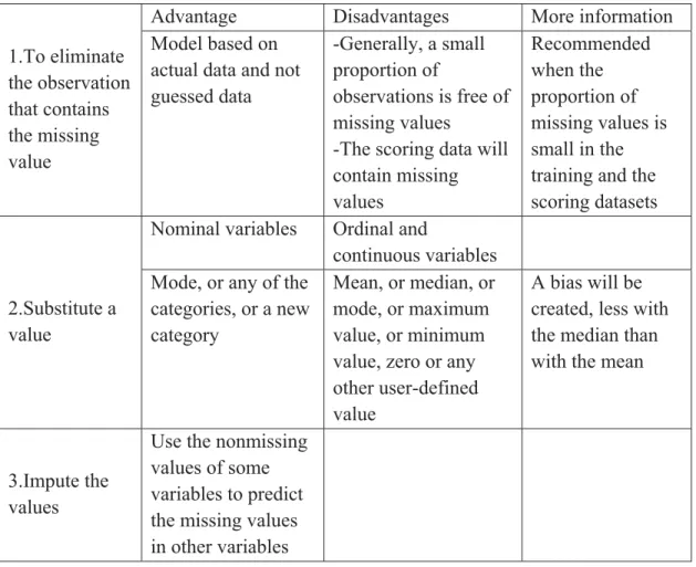
3.2.1 Missing values ... 51
3.2.2 Data transformations... 55
3.2.3 Normalization of the data ... 55
3.2.4. Variable reduction ... 57
3.2.5 Variables selection ... 59
3.2.6 A checklist ... 63
3.3. Different data sets for different models ... 64
4.1 Logistic regression ... 74
4.1.1 Overview ... 74
4.1.2 Multicollinearity ... 77
4.2 Decision trees ... 78
4.2.1 Overview ... 78
4.2.2 Developing an initial tree ... 80
4.2.2.1 Entropy ... 82
4.2.3 Pruning the tree through the validation data ... 83
4.2.4 Advantages and weaknesses of decision trees ... 85
4.3 Neural networks ... 87
4.3.1 Overview ... 87
4.3.2 Description of a neural network model ... 88
4.3.3 The output layer ... 90
4.3.4 How are the weights estimated in every unit? ... 92
4.3.5 Advantages and weaknesses of neural networks ... 94
Chapter 5: Results and evaluation of the predictive models ... 97
5.1 Overall Fit ... 97
5.2 Results of the logistic regression models for the different data sets ... 98
5.3 Probability of default using logistic regression ... 124
5.4 Results of the decision tree models for the different sets ... 129
5.5 Results of the neural networks ... 138
5.6 Comparative results between the three methods ... 139
5.7 The predictive power of the Receiver Operating Characteristic Charts ... 141
Chapter 6: Summary and conclusions ... 152
List of figures
Figure 2.1: “Hypothetical Agricultural Loan Requests” (Featherstone, et al. 2007, 21) .... 7
Figure 2.2: The five categories that constitute the components of a FICO score (myFICO 2010) ... 8
Figure 2.3: "Causes of Crop Losses" (Baquet, Hambleton and Jose 1997, 13) ... 11
Figure 2.4: "Farm Credit System Loan Portfolio" (Steeves 2009, 16). ... 13
Figure 2.5: "Sources of Borrowed Capital, Largest Cooperatives Compared with All Others, Fiscal 1987” (Royer, Wissman and Kraenzle 1990, 39) ... 14
Figure 2.6: “The Probability Density Function of Loan Losses” (Zech and Pederson 2004, 93) ... 18
Figure 2.7: "Activities that compose the KDD process” (Fayyad et al. 1996; Arns Steiner, et al. 2006, 7) ... 27
Figure 2.8: “The agricultural lending decision structure” (Bryant 2001, 80) ... 35
Figure 2.9: “Lender preferences for combinations of loan characteristics” (Barry, et al. 2000) ... 43
Figure 4.1: An example of a tree for the target variable default ... 79
Figure 4.2: A neural network with two hidden layers ... 89
Figure 5.1: Decision tree for the 2006 - 2010 (11) data set ... 131
Figure 5.2: Decision tree for the 2006 - 2010 (12) data set (First half) ... 132
Figure 5.3: Decision tree for the 2006 - 2010 (12) data set (Second half) ... 132
Figure 5.4: Decision tree for the 2006 - 2010 (21) data set ... 133
Figure 5.5: Decision tree for the 2006 - 2010 (22) data set ... 133
Figure 5.6: Decision tree for the 2007 - 2010 (11) data set ... 134
Figure 5.7: Decision tree for the 2007 - 2010 (12) data set ... 135
Figure 5.8: Decision tree for the 2007 - 2010 (21) data set ... 136
Figure 5.9: Decision tree for the 2007 - 2010 (22) data set ... 137
Figure 5.10: ROC charts for the 2006 (1) data set ... 143
Figure 5.11: ROC charts for the 2006 - 2010 (11) data set... 144
Figure 5.12: ROC charts for the 2006 - 2010 (12) data set... 145
Figure 5.14: ROC charts for the 2006 - 2010 (22) data set... 147
Figure 5.15: ROC charts for the 2007 - 2010 (11) data set... 148
Figure 5.16: ROC charts for the 2007 - 2010 (12) data set... 149
Figure 5.17: ROC charts for the 2007 - 2010 (21) data set... 150
Figure 5.18: ROC charts for the 2007 - 2010 (22) data set... 151
Figure 6.1: A diagram to decide the appropriate model to be used to calculate the probability of default... 153
List of tables
Table 2.1: Information on Type I and Type II errors ... 21
Table 2.2: Articles that apply neural networks in accounting and finance (Paliwal and Kumar 2009) ... 25
Table 2.3: Abbreviations used in table 2.2 (Paliwal and Kumar 2009) ... 26
Table 2.4:"Summary of Financial Ratios Used in the Seven Noted Failure-Predictive Models, Including Model Method, Failure Definition, and Industry Studied" (Gallagher 2001) ... 29
Table 2.4: (Continued) ... 30
Table 2.5: Summary of the quantitative variables used in evaluating agricultural loans (Bryant 2001) ... 33
Table 3.1: The list of independent variables ... 48
Table 3.1: (Continued) ... 49
Table 3.1: (Continued) ... 50
Table 3.2: Strategies to treat missing values ... 53
Table 3.3: Summary of imputation methods (Refaat 2007) ... 54
Table 3.4: The different sets ... 69
Table 3.4: (Continued) ... 70
Table 3.4: (Continued) ... 71
Table 3.4: (Continued) ... 72
Table 4.1: Profits and losses from assessment decisions ... 80
Table 4.2: Profit matrix ... 84
Table 5.1: Logistic regression results for the 2006 (1) data set ... 99
Table 5.2: Logistic regression results for the 2006 - 2010 (11) data set ... 101
Table 5.2: (Continued) ... 102
Table 5.3: Logistic regression results for the 2006 - 2010 (12) data set ... 103
Table 5.3: (Continued) ... 104
Table 5.3: (Continued) ... 105
Table 5.4: Logistic regression results for the 2006 - 2010 (21) data set ... 106
Table 5.5: Logistic regression results for the 2006 - 2010 (22) data set ... 108
Table 5.5: (Continued) ... 109
Table 5.5: (Continued) ... 110
Table 5.6: Logistic regression results for the 2007 - 2010 (11) data set ... 111
Table 5.6: (Continued) ... 112
Table 5.6: (Continued) ... 113
Table 5.7: Logistic regression results for the 2007 - 2010 (12) data set ... 114
Table 5.7: (Continued) ... 115
Table 5.7: (Continued) ... 116
Table 5.7: (Continued) ... 117
Table 5.8: Logistic regression results for the 2007 - 2010 (21) data set ... 118
Table 5.9: Logistic regression results for the 2007 - 2010 (22) data set ... 119
Table 5.9: (Continued) ... 120
Table 5.9: (Continued) ... 121
Table 5.9: (Continued) ... 122
Table 5.10: Example of the normalized data of two customers ... 128
Table 5.11: Comparative results between the different models for the different sets of data ... 140
Table 5.11: (Continued) ... 141
Chapter 1: Introduction
Farmers need money to be able to run their businesses, to change their equipment, buy seeds, fertilizers and other inputs, and pay for labor and other expenses. Many financial institutions offer loans to farmers. Those financial institutions aim to generate profit from the interest rate charged on each loan. Their concern is not to lend to farmers who will not pay back the loan, as they will lose part of the capital, and the interest. They will also acquire losses that offset the benefits acquired from several other borrowers. For this reason, every financial institution providing loans to farmers has a continuous incentive to create a better mechanism for assessment of borrowers. For a financial lending institution, some questions remain not fully answered. How much knowledge can the financial institution extract from the data stored throughout the years? Can the original financial and non-financial data provided by the borrower indicate the probability of the loan to default and which can potentially help in the decision of approving the loan? And what is the potential information that needs to be stored for future analytical use? This study intends to provide a contribution to answer those questions since financial lending institutions aim to continuously improve their credit assessment models to increase the level of prediction accuracy which will potentially lead to a decrease in their portfolio exposure to credit risk.
1.1 Statement of the problem
The granting of loans by creditors is a challenging decision with the current economic crisis. Back in 1973, Conley (1) states that “the years 1972 and 1973 will long be remembered as being unique in the history of U.S. grain marketing”. He stated
several events and I will mention two of them:
1. The U.S. sold wheat and other grains in relatively large amounts to Russia and mainland China. This induced higher prices, but many farmers were not able to benefit from the export subsidies paid as they had sold their grain already.
2. The increase in demand for soybeans.
In 2006, 2007 grain producers did benefit from higher prices compared to previous years and those years will long be remembered as well. Would looking to the farm borrower loan pay back and default be similar before and after this period?
For the creditors it is of great importance to assess correctly the risk profile of all applicants for credit. The capacity to differentiate between customers is crucial. The refusal of good credit can cause the loss of future profit margins (commercial risk) and the approval of bad credit can cause the loss of the interest and the principal money (credit risk). The losses might have been reduced through full knowledge of the loan characteristics and a better credit risk evaluation system.
Consequently, a reliable model that predicts defaults accurately is imperative. Creditors should base their decision on a reliable model to make some corrective or predictive measures. An accurate credit risk assessment will allow the creditors to make a better request for collateral corresponding to the risk, to price the loan
correspondingly, to decide which loans need special monitoring, and to evaluate the agricultural loan portfolio of a financial institution.
As a result, there is a need to build models that help in credit classification. Those models are generally based on large past databases of loans that support the decision process. Those models will also classify loan applications into good and bad applications. A good application is the one that belongs to an applicant that is credible to be given a loan, and a bad application is an application that should be rejected due to the probability of the applicant not returning the loan. The results describe feasible and handy models that can be economically adopted by financial institutions serving the agricultural sector.
1.2 Objectives and significance of the study
A major source of risk encountered by an agricultural lending financial institution is credit risk. It accounts for the risk of loss from agricultural loan defaults. Several objectives are to be achieved through the classification and prediction of agricultural loans default. Those objectives can be summarized as follows:
1. Identify the financial and non-financial variables that signal the capacity of borrowers to pay back the loan, and
2. Determine the best model(s) to evaluate credit risk.
These objectives were achieved through the use of logistic regression, decision trees, and neural network, to determine the predictive accuracy of each method after using different samples for training, validation and testing. The benefits of the models
suggested are in their capacity to provide a better credit risk assessment which, when combined with the convenient decision process, will potentially lead to a better
allocation of the financial institution’s capital.
The aim of this study is to provide an additional tool that helps in reducing the proportion of unsafe borrowers which will have a positive effect on the financial institution. Due to the significance of credit risk analysis, this study was done to add additional information to the agricultural loan decision-making process, potentially decrease the cost and time of appraisal of loan applications, and decrease the level of uncertainty for loan officers by providing knowledge extracted from previous loans. The extraction of knowledge was done through the examination of both financial and non-financial criteria of the business, and of the operator, to identify the credit risk.
1.3 Organization of the study
The remainder of the study is organized as follows. A background section about credit risk evaluation and a literature review follows the introduction. Chapter Three presents the data used and the data preparation process. In Chapter Four the methods are reviewed, explained and discussed. Chapter Five describes the results and compares the methods adopted. Chapter Six states some concluding remarks and directions for further future research.
Chapter 2: Background and literature review
2.1 Previous studies
Several studies looked at the evaluation of agricultural loan applications. One of the studies examined the characteristics and performance of 87 credit scoring models that were used by lenders (Ellinger, Splett and Barry 1992). Their target was to measure the consistency among the models. They found a lack of a uniform model or models that can be used by lenders to evaluate the creditworthiness of agricultural borrowers. Furthermore, the predictive accuracies of four alternative credit scoring models (the linear probability model, discriminate analysis, logit and probit) have been analyzed by Turvey (1991). He used loan application data from Canada’s Farm Credit
Corporation. The findings did not show a great deal of predictive accuracies in the four model types (between 71.5% and 67.1%) but stresses the importance of inclusion of both qualitative and quantitative attributes when choosing the credit scoring model. Another study looked at 157,853 loans in the seventh Farm Credit District Portfolio. The results of the study show the accuracy of financial performance ratios (repayment capacity, owner equity, and working capital origination loans) in calculating the expected probability of default (Featherstone, Roessler and Barry 2006). Featherstone, et al. (2007) used data from a survey that they conducted in Kansas and Indiana to explore the agricultural lending process. Their main targets were to investigate the factors (financial, non-financial information, borrower and lender characteristics) used by financial institutions when deciding the approval of the loans requested by farm borrowers and the interest rates. They used tobit models to
generate a loan approval decision model and OLS models to determine the interest rates presented to farm borrowers.
Featherstone, et al. (2007) used the credit-scoring model of Featherstone, Roessler and Barry (2006) to calculate the log odds ratio in order to determine the probability of default (credit risk). The log odds ratio used is equal to:
ܮ݊ ቀ ௧௬௨௧
ଵି௧௬௨௧ቁ ൌ െʹǤ͵Ͷ͵ െ ͲǤͲͲͳ͵ͷሺܴܥሻ െ ͲǤͲʹͳሺܱܧሻ െ
ͲǤͲͲ͵ͻͻሺܹܥሻ ሺʹǤͳሻ
The independent variables are as follows: RC represents the repayment capacity percentage, OE is the owner equity percentage, and WC is the working capital percentage. The calculation of the probability of default now becomes possible;
ൌ ୣ౮ౘ
ଵାୣ౮ౘ (2.2)
where xb is the result of the right hand side of the equation of the log odds ratio.
The lending factors used in the study of Featherstone, et al. (2007) are character, Fair Isaac credit bureau score (“a quantitative nonfinancial variable that provides an indication of the borrower’s financial integrity” p.19), financial record keeping, productive standing, and credit risk. An example of four hypothetical agricultural loan requests can be summarized in figure 2.1 below:
Figure 2.1: “Hypothetical Agricultural Loan Requests” (Featherstone, et al. 2007, 21)
LQ, MID, and UQ refer to Lower Quartile, Mid Quartile and Upper Quartile, respectively.
Financial Record Keeping
725 poor 1 → Farmer Dixon
Fair Isaac Credit Bureau Score Productive Standing MID Credit Risk Honest 560 Financial Record Keeping Avg. Productive Standing LQ 2 → Farmer Hudson Character Productive Standing Credit Risk Exc. LQ Financial Record Keeping Credit Risk
Dishonest 725 3 → Farmer Morgan
Fair Isaac Credit Bureau Score 560 Financial Record Keeping Credit Risk
Poor UQ 4 → Farmer Wells
Productive Standing
A description of the five elements that determine the Fair Isaac Credit Bureau Score (FICO) is provided in figure 2.2 below:
Figure 2.2: The five categories that constitute the components of a FICO score (myFICO 2010)
Their findings are that the experience of the loan officers (in years) negatively affects the proportion of loan granted (Featherstone, et al. 2007). In addition, the amount of time (in hours) spent by loan officers on agricultural loans had a positive impact on the proportion granted. Furthermore, the results of the middle productive standing variable are higher than the upper quartile productive standing which may imply that productive standing is important to avoid borrowers in the lower quartile. They also state that it may imply that productive standing is not an important factor in the agricultural loan decision-making. Additionally, FICO has a large impact on the proportion granted. Moreover, their expected results show that as the borrower’s
35% 30% 15% 10% 10% Payment History Amounts owed
Length of credit history New credit
financial record abilities increase, the proportion of the approved loan increased. Even though credit bureau scores are present, the majority of studies do not explicitly show how the lenders use this information when lending to farm borrowers (Featherstone, et al. 2007).
The results of a study done by Perry (2008) that uses data from a national survey of
consumers’ shows those consumers with higher credit scores had “higher incomes”, and “higher levels of education”. Those consumers with higher credit scores were older than the consumers “with low credit scores”, less likely to have previously had “major medical expenses”, or have been unemployed or have had a decrease in their income during the past two years. Iyer, et al. (2009) provided evidence based on their data in their study on creditworthiness in peer-to-peer markets that credit score captures a dimension of creditworthiness through the prediction of actual borrower default behavior. They also state that limiting our thinking to the individual credit score of the borrower when assessing the creditworthiness is inaccurate.
For a multitude of reasons, creditors have faced difficulties over the years. The major cause of serious banking and related systems problems continue to be directly related to negligent credit standards for borrowers, poor portfolio risk management, or a lack of attention given to changes in economic or other circumstances. In general, capital budgeting techniques (such as Interest Rate of Return (IRR), Net Present Value (NPV), Benefit/Cost B/C ratios, etc.) are used in the ranking selection and acceptance procedure of an investment project. Those techniques assume that the decision
production, factor costs and other valuable variables” (Philippatos 1974, 104). According to Philippatos (1974), under certainty characterized by complete information, each alternative faced by the decision maker has a unique outcome. Conversely, when we include realism in conducting the analysis, we must allow measures of uncertainty associated with all future expectations (Philippatos 1974). He states that in the scenarios where the probabilities of possible outcomes are known by the decision maker, those scenarios are characterized by risk. According to Prakash, Karels and Fernandez (1987, 132) there are several inputs needed to make a capital budgeting decision under certainty. They can be summarized as follows:
1. “The determination of the effect of working capital on cash flow
2. Estimation of the life of the project
3. Estimation of the initial investment
4. Estimation of net income
5. Estimation of cash flow
6. Determining the cost of capital”
Under uncertainty, the authors suggest that the inputs included in the calculation of
the cash flow “need to be adjusted to account for the riskiness of the projects”
(Prakash, Karels and Fernandez 1987, 187). Baquet, Hambleton and Jose (1997, 3)
mention five primary sources of risk faced by farmers: “Production”, “Marketing”, “Finance”, “Legal”, “and Human Resources”. At the same time, they refer that
farmers are not competing alone as they do have several entities they can count on for advice and include that advice in their planning. They have stated in the pie chart in figure 2.3 below the share of the causes of crop loss.
Figure 2.3: "Causes of Crop Losses" (Baquet, Hambleton and Jose 1997, 13)
Baquet, Hambleton and Jose suggest that the objective of the farmer shall be to manage risk through sound planning and financial control. Additionally, they state that even if the interest may be out of control of the farmer, the farmer can sometimes utilize crop insurance with a marketing plan to decrease the debt-to-asset ratio which
can influence the interest rate charged. Adopting this suggestion reduces the lender’s
risk exposure (Baquet, Hambleton and Jose 1997). Drought and Heat 47% Excess Moisture 22% Cold, Frost, Freeze13% 9% 3% 2% 2% 1% 1%
Drought and Heat Excess Moisture Cold, Frost, Freeze Hail Disease Wind, Hurricane Flood Insects Other
Diversification in crop production can reduce the risk and instability of farm income (Newbery and Stiglitz 1999; Mishra, El-Osta and Steele 1999). Additionally, the financial performance variability of projects that adopt a diversification between crop and livestock production is less. Mishra, El-Osta and Steele (1999) figured out from
the study they conducted on “Factors Affecting the Profitability of Limited Resource and Other Small Farms” that sole proprietorships were more profitable than farms legally organized differently. Furthermore, they found that farmers who bought crop insurance have higher earnings when compared to the other farmers who did not buy crop insurance. They suggest that beginning farmers and limited resource farmers could increase the farm profitability through the decrease in the need for capital financing by leasing farm land and farm equipment. Along with that, operators with less than 10 years of experience in business operations are characterized by a lower level of equity and higher debt to asset ratios (Mishra, Wilson and Williams 2009). Moreover, Nwoha, et al. (2007) stated that the Farm Service Agency (FSA) is one destination for farmers characterized by low solvency and liquidity and who are deprived of credit from commercial sources to ask for assistance.
Dodson and Koenig (2004) found from the logistic regression results that Farm Credit Services (FCS) serve larger farming operations where the hobby and part time market were more likely being served by banks. Their multivariate logit analysis results show that the borrowers served by FCS belong to a different segment than the borrowers getting services by commercial banks. Steeves (2009) writes about the battle between community banks and the farm credit system. He states that the farm credit system and its associations are seen as the real loan competitors rather than regional banks.
He states the example of a bank owner who had to go to the Farm Credit System to get millions of dollars because it is a large loan and because of the lower interest rate offered that cannot be beaten even by larger banks. Additionally, Steeves mentions that the loan portfolio of the Farm Credit System grew from $82.6 billion to $161.4 billion between the year 2001 and 2008 and can be divided according to figure 2.4 below as of December 2008.
Figure 2.4: "Farm Credit System Loan Portfolio" (Steeves 2009, 16).
Mentioning the large figures, it might be interesting to look a few years back to find the sources of money that were used by cooperatives. A study on farmer cooperatives
shows that “the proportion of borrowed capital supplied by commercial banks Rural real estate loans 3% Communication loans 3% Other 4% Real estate mortgage loans 44% Production and intermediate-term loans 23% Agribusiness loans 17% Energy and water/waste disposal loans 6%
Rural real estate loans
Communication loans
Other
Real estate mortgage loans
Production and
intermediate-term loans Agribusiness loans
Energy and water/waste disposal loans
generally decreases as size increases” (Royer, Wissman and Kraenzle 1990, 35). They showed in figure 2.5 the sources of borrowed capital used by cooperatives.
Figure 2.5: "Sources of Borrowed Capital, Largest Cooperatives Compared with All Others, Fiscal 1987” (Royer, Wissman and Kraenzle 1990, 39)
Nevertheless, they also state that for the cooperatives with assets ranging from $25
million to $100 million, there was a remarkable “increase in the proportion of
borrowed capital provided by commercial banks to cooperatives (Royer, Wissman and Kraenzle 1990, 35).
Loan officers hired by creditors to make decisions on accepting or rejecting applications are given some instructions to assess loan applications and after a certain period of time they gain some intuition or acquire some personal knowledge in deciding whether an application is loan worthy or not. It is well known that the capacity of humans to make successful credit evaluations is poor (Glorfeld and Hardgrave 1996).
19.30% 9.70%
61.40% 9.50%
Cooperatives with less than $500 million assets Other sources Bonds & notes Banks for Cooperatives Commercial banks 39.20 % 25.10 % 30.20 % 5.60%
Cooperatives with more than $500 million assets
Levy and Benita (2009) test the subjectively weighted probabilities to equally likely outcomes to know whether subjects have a systematic cognitive bias and whether the bias (in case it exists) influences their behavior. Their results show that subjects accord a considerably higher weight to moderate outcomes in comparison to extreme outcomes for positive, negative and mixed prospects; the distribution of outcomes they found is very uneven. Their explanations for this phenomenon are as follows:
1. Individuals consider that extreme outcome events are less likely due to the deeply rooted notion of a bell-shaped distribution
2. Individuals prefer not to go far in their guesses 3. some inclination for optimism
Taking into consideration the fact that humans are not good at finding the necessary relationships and accord higher consideration to moderate outcomes, it is important to rely on a different tool. Previous studies show that knowledge discovery, a branch of data mining, “provides a variety of useful tools to discover the non-obvious relationships in historical data, while ensuring the generalization of those relationships to the new/future data” (Bigus 1996; Marakas 1999; Handzic, Tjandrawibawa and Yeo 2003, 98). The outcome can be used by the loan officers as an additional tool in deciding whether to approve or decline loan requests (Handzic, Tjandrawibawa and Yeo 2003). They argue as well that neural networks are a suitable knowledge discovery tool that can help loan officers for this purpose.
Gustafson, Beyer and Saxowsky (1991) looked to the ways loan officers treat the information collected to decide on the approval of providing credit. Their reasoning is
based on the fact that with experience, loan officers acquire lending heuristics which increase their accuracy and speed of credit evaluations. They surveyed ten agricultural lenders each with at least five years of lending experience in the same area and their findings can be summarized as follows: all lenders acknowledged the importance of solvency, whereas 80% of the lenders accorded importance to liquidity ratios. Moreover, lenders did also accord great importance to the characteristics of the borrower mainly: honesty, integrity and production management ability (Gustafson, Beyer and Saxowsky 1991). Barry, et al. (2000) mention that the lender-borrower relationships do not substitute consideration to the interest rate charged or to the credit risk evaluation; besides, they will influence the soundness of the loan and they may help decrease the administrative expenses of lending. The absence of one of the three characteristics of “honesty”, “integrity”, and “reliability” can decrease the credit
limit to zero (Barry, et al. 2000). Gloy, LaDue and Gunde (2005) state that the nonfinancial variables elaborated by lenders through subjectively assessing the
borrower’s character, commitment to repay, management capacity, and future
business prospects play a major role in the evaluation and approval of a loan application. Based on the information available to the loan officers and their relationship with the customer, loan officers can identify the major reasons for declining their loan application and can suggest to the borrower some steps that he/she could take to help in making a more accurate credit decision; this step will reduce the waiting time of the borrower and decrease the risk of losing the operation (Arns Steiner, et al. 2006).
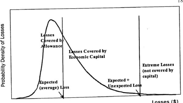
In general, lenders use benchmarks for financial ratios, collateral margin minimums and other guidelines that they have developed as lending standards (Gallagher 2001). When lenders approve a loan and the borrower fails to return the money, numerous costs are incurred by the financial lending institution. Featherstone and Boessen (1994) mention that credit scoring models have been used to analyze the probability of default; those models do not account for the loss associated with default which is more of an interest to investors at the portfolio level rather than the individual level. Gustafson, Pederson and Gloy (2005) mentioned the following types of losses: personnel time and resources, the loss from interest that has not been accrued and uncollected accounts receivables related to agricultural debt offs. Those losses might have been reduced through full knowledge of the loan characteristics and a better credit risk evaluation system. Zech and Pederson (2004) estimate “the distribution of loan losses due to credit risk” for a portfolio, which is shown in figure 2.6 below.
Figure 2.6: “The Probability Density Function of Loan Losses” (Zech and Pederson 2004, 93)
The distribution they present is continuous, smooth and has a fat right tail. It shows that the occurrence of big losses has a low probability (Zech and Pederson 2004). They mention that the silhouette of the probability distribution function of the
portfolio depends on several factors: “loan default probabilities, relative loan sizes,
correlations of default between loans, and concentrations by the number of loans and
sectors” (Zech and Pederson 2004, 93). They calculate the expected loss of a loan by following this formula:
EL=EAD*PD*LGD (2.3)
where EL ($) stands for Expected Loss; EAD stands for Exposure At Default ($),
Probability of Default (%); and LGD represents the Loss Given Default (%), which is
“the amount that is net of loan loss recovery in the case of default”.
Turvey (1991) studied four alternative credit scoring models, linear probability, discriminant analysis, logit, and probit models based on 9,403 loan applications from
the Canada’s Farm Credit Corporation. His findings do not show a big difference in the predictive accuracies of the four mentioned models which ranged between 71.5% logit to 67.1% for the linear probability model. He stressed the point that both quantitative and qualitative considerations shall be attributed when it comes to the choice of one model instead of the other. Ellinger, Splett and Barry (1992) measured the characteristics and consistency of 87 credit scoring models used by agricultural lenders through the use of 324 simulated loan cases with different financial characteristics and risk levels. They stated that there are several reasons behind differences in credit scoring models. Their statement of this difference has been explained as follows:
1. Different purposes can be achieved through credit scoring models depending on the decision process of the lender,
2. Different lenders have different risk attitudes,
3. Different lenders have different types of borrowers and different types of information available.
Their findings emphasize the enduring absence of unique model(s) to evaluate the credit risk of agricultural borrowers and the need of more interchange between lenders and borrowers.
Ziari, Leatham and Turvey (1995) applied in their study on credit scoring of
agricultural loans both parametric (statistical) discriminant models (logit and Fisher’s
linear discriminant model) and mathematical programming as a non parametric method. They stated several reasons why non-parametric discriminant analysis like neural networks and mathematical programming could be used. They state, for example, that those methods do not require the assumption that misclassification costs arising from Type I and Type II errors are the same, and they can resolve complex discrimination problems. Their conclusions prove that mathematical programming models can perform as well as the statistical models. Rambaldi, Zapata and Christy (1992) mention that from a banker’s perspective, a Type I error in classifying will incur a higher cost than the Type II error. Additionally, when lenders face applications for investments with the same level of risk, they prefer to lend the money to the less risk-averse farmer (Wang, Leatham and Chaisantikulawat 2002). The most damaging decision is the one that misclassifies the non-worthy loan application as loan worthy, which means the financial institution is providing loans to the non-worthy borrowers (Handzic, Tjandrawibawa and Yeo 2003).
A Type I error occurs when the financial institution incorrectly assigns to a loan application a lower level of risk. In this situation the financial institution incurs some losses due to default and possibly losses because the amount of collateral requested was lower than needed. While a Type II error occurs when the financial institution incorrectly considers a loan application as a high level of risk application. In this situation the financial institution will lose some potential revenue. The desire is to improve the performance of the decision model through the techniques suggested. To
avoid the trade-off between pursuing the best performance on negative misclassified data and the best performance on all data, it is suggested to include a weight for every decision and maximize profit of the financial institution. A description of the two types of errors is provided in table 2.1 below.
Table 2.1: Information on Type I and Type II errors
Assessment by Financial Institution Capable of paying back
the loan
Incapable of paying back the loan
Borrower
Capable of paying back the loan
$ Benefit to the institution
$ Loss to the institution Type I Incapable of paying
back the loan
$ Loss to the institution Type II
$0 (or to include the cost from screening)
Admitting the presence of the two types of errors, it is very important to have an excellent agricultural credit risk evaluation. Glorfeld and Hardgrave (1996) state that several studies proved that analytical neural networks are successful in bankruptcy prediction; the neural networks learn by examples, from very noisy, distorted, or incomplete data and can adjust dynamically to fit the data where other methods fail.
They aimed to model the loan committee’s decision to approve or decline a loan request. The classification of a loan application can be described as follows:
1. A good application is well classified
2. A good application is misclassified and then rejected
3. A bad application is approved to get a loan
There are four important measures to assess misclassification:
1. “Accuracy: (true positives and negatives) / (total cases) (2.4) 2. Error rate: (false positives and negatives) / (total cases) (2.5) 3. Sensitivity: (true positives) / (total actual positives) (2.6) 4. Specificity: (true negatives) / (total actual negatives)” (Siddiqi 2006, 120). (2.7)
Another study (Handzic, Tjandrawibawa and Yeo 2003, 97) illuminates several reasons for which the capacity of loan officers to judge the creditworthiness is poor;
(1) “the presence of a large gray area where the officers will make a subjective decision”; (2) “humans have a tendency to be biased, and personal relationships or familiarity with the applicants might twist the judgmental aptitude”; and (3) “the historical data from the previous applications surely contain much hidden knowledge that may be utilized in supporting the decision-making”. Additionally, humans find difficulties in discovering patterns and relationships from data because of the large volume of the data and because of the non-obvious nature of the relationships (Handzic 2001; Handzic, Tjandrawibawa and Yeo 2003). Artificial intelligence techniques, especially machine learning techniques such as neural networks have been used in default prediction and bankruptcy prediction as well as credit rating analysis (Huang, et al. 2004). Phillips and Katchova (2004) examined the change in credit score migration rates probabilities across business cycles (which may be used as proxy for the systematic risk). They follow the classification of business cycles of the published reports of the National Bureau of Economic Research. Their results from cycles suggest “farm businesses exhibit a higher tendency to downgrade
(upgrade) than upgrade (downgrade) during recessions (expansions)” but they did not find trend reversal in agricultural borrowers (Phillips and Katchova 2004, 13). Gloy, LaDue and Gunde (2005, 15) looked at credit risk migration and downgrading. One of their findings shows that the least likely borrowers to face credit risk downgrade
are “the borrowers at the level of retiring” and the ones that are “actively involved in
their business but with children past college age”.
Gallagher (2001) used a theoretical model to distinguish between unsuccessful and successful agribusiness loans that included the lender experience and the model is stated as follows: “Agribusiness Loan Success = f(Leverage, Liquidity, Coverage, Activity, Efficiency, Business Age, Manager Experience, Lender Experience, Use of
Financial Advisor)” (Gallagher 2001, 24). He assumes that the coverage ratio captures some of the important economic conditions that are significant to the success of an agribusiness. Gallagher (2001) used primary loan data that contains financial and non-financial variables and applied the logistic regression method to differentiate between successful and non-successful agribusiness loans. He found that unsuccessful
loans were associated with “less experienced primary and supervisory loan officers,
and repayment projections prepared more often by the borrower or accountant”
(Gallagher 2001, 32). Kao and Chiu (2001) state that the classification and regression tree (CART) and the analytical neural networks provide an alternative to logistic regression especially when the relationships between dependent and independent attributes are highly nonlinear. Their decision to use CART is based on a previous study that proved that CART is essentially non-parametric. Satchidananda and Simha (2006) used data from two banks in India that provide agricultural production loans to
farmers. They examined two classifiers: logistic regression and decision trees. They state that decision trees have been considered as white-boxes, compared and evaluated the accuracy and efficacy of the two classifiers. They acknowledge the universal approximation property of neural networks in credit scoring and state its lack of explanation capability when used for decision-making. Artificial intelligence
researchers studied two approaches for classification problems: the “symbolic approach” based on decision trees and the “connectionist approach” which is mainly
based on neural networks (Arns Steiner et al. 2006). Neural networks are not new to economics and finance; in fact they have been used to solve problems in these areas previously (Vellido, Lisboa, & Vaughan 1999; Angelini, Tollo and Roli 2008). Problems solved with neural networks can have different forms: classification and discrimination, function approximation and optimization, and series prediction (Angelini, Tollo and Roli 2008). Paliwal and Kumar (2009) did a thorough review of the application of neural networks. Ninety-six studies compare neural networks with regression analysis, logistic regression, and discriminant analysis applied in the field of accounting and finance, health and medicine, engineering and manufacturing, marketing, and general applications. A list of the articles they mentioned where neural networks have been applied in the area of accounting and finance is revealed in table 2.2 below.
Table 2.2: Articles that apply neural networks in accounting and finance (Paliwal and Kumar 2009)
Reference Statistical model
No. of
variables Sample size
Validation
method Error measure Finding Odom and Sharda (1990) DA 5 129 Tr-Ts/R-3 times Confusion matrix [A] Duliba (1991) Reg 10-May 600 Tr-Ts R2 Value [A]-Random effect [C]-Fixed effect Salchenberger
et al. (1992) Logit 29 3479 Tr-Va-Ts
Confusion
matrix [A]* Tam and Kiang
(1992) k-NN, DA,ID3 19 118 Jackknifing Confusion matrix [A] Fletcher and Goss (1993) LR 3 36 18-fold CV Confusion
matrix, MSE [A] Yoon et al. (1993) DA 4 151 Tr-Ts (50-50) Confusion matrix [A] Altman et al. (1994) DA 10-DA 15-NN 1108 Tr-Ts (70-30) Confusion matrix [C] Dutta et al. (1994) Reg, LR 6, 10 47 Tr-Ts (70-30) Confusion matrix [A] Wilson and Sharda (1994) DA 5 129 Tr-Ts/R-3 times Confusion matrix [A]* Boritz and Kennedy (1995) Logit, Probit, DA 5, 9 342 Tr-Ts (70-30) / R-5 times Confusion matrix [B] Lenard et al. (1995) LR 4 & 8 80 Tr-Ts (50-50) Confusion matrix [A]* Desai et al. (1996) LR, DA 18 2733 Tr-Ts (70-30) / R-10 times Confusion matrix [B]* Leshno and Spector (1996) DA 41 88 Tr-Ts Confusion matrix [A]* Jo et al. (1997) DA,CBR 20 564 Tr-Ts Confusion matrix [A]* Spear and Leis
(1997) DA, LR, Reg 4 328 Tr-Va-Ts (76-12-12) Confusion matrix [B] Zhang et al. (1999) LR 6 220 5 fold CV Confusion matrix [A]*
Lee and Jung (2000) LR 11 21678 Tr-Ts C-index, Some measure for degree of separation [A]-Rural customer [C]-Urban customer Limsombunchai et al. (2005) LR 11 16560 Tr-Ts Confusion matrix [B] Lee et al. (2005) DA, LR 5 168 4 fold CV Confusion matrix [A]* Pendharkar (2005) C4.5, DA 3 100-sim 200-real Bootstrapping Confusion matrix [A]* Landaja et al. (2007) Robust reg.
A summary of the performance of neural networks is stated as follows: multilayered feed forward neural network outperformed in about 58% of the cases, and in the rest of the cases it performed equivalently to the traditional statistical methods (24%) and in 18% of the cases traditional statistical methods outperformed (Paliwal and Kumar 2009). Additionally, they mentioned that the statistical methods are based on assumptions and consequently the validity of their performance will be essential. Another point mentioned in their findings is related to the size of the data set and the number of variables used, which have been very different between the different studies. An explanation of the abbreviations used in table 2.2 is provided in table 2.3.
Table 2.3: Abbreviations used in table 2.2 (Paliwal and Kumar 2009)
Notation Meaning
Reg Regression Analysis
LR Logistic Regression
DA Discriminant Analysis
CBR Case Based Reasoning
CART Classification and Regression Tool
DT Decision Tree
k-NN k-Nearest Neighbor
Tr-Ts Training set - Test set
Tr-Va-Ts Training-Validation-Test data sets n-fold CV n-fold Cross Validation
R-n Procedure Repeated n number of times
RMSE/MSE Root Mean Square Error / Mean Square Error
MAE Mean Absolute Error
[A] Neural network's performance is better
[B] Performance of both the methods are equivalent [C] Statistical technique's performance is better
* Studies where some statistical test has been carried out to compare the results from various techniques
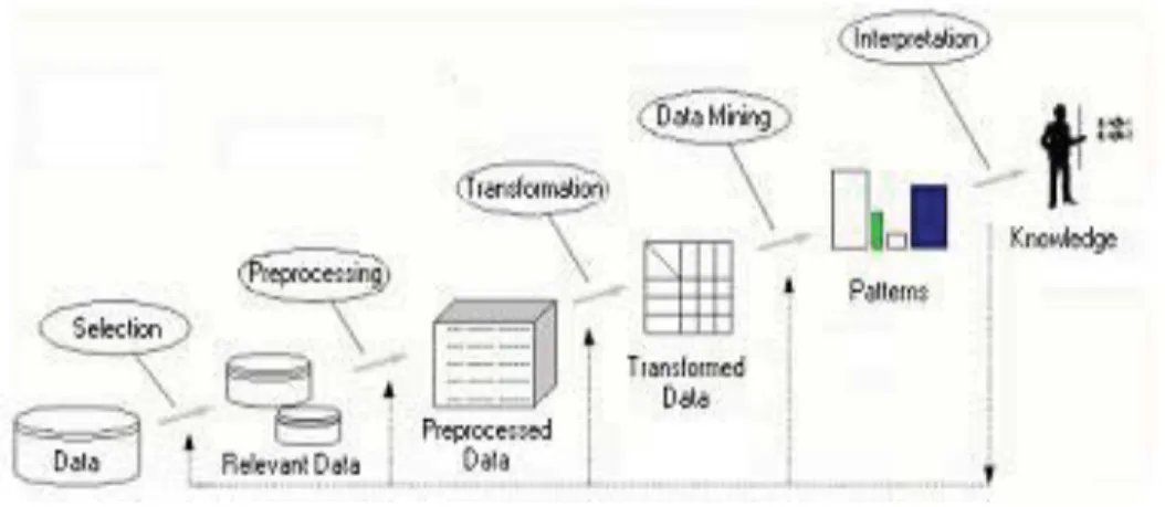
Odeh, Featherstone and Das (2010) used an artificial intelligence method along with existing methods to predict credit default and assess the economic consequences of the forecast of each model. They used data from 157,853 loans from eleven states from the 1995-2002 period. Their findings show that a different method performed best when comparing out-of-sample and in-sample performance. Logistic regression performed best in out-of-sample prediction while the adaptive neuro-fuzzy inference system had the highest in-sample accuracy (Odeh, Featherstone and Das 2010). In simple words and with the help of the illustration 2.7 below, the process of Knowledge Discovery in Databases (KDD) is described and the description is based on the work of Arns Steiner, et al. (2006). The process consists of five steps: “data selection”, “data pre-processing and cleaning”, “data transformation”, “data mining”, “and result interpretation and evaluation”.
Figure 2.7: "Activities that compose the KDD process” (Fayyad et al. 1996; Arns Steiner, et al. 2006, 7)
Noticeably, the first important step in the process is data selection. The next section is devoted to reviewing some studies which will provide direction when choosing variables.
2.2 Choice of variables
Gallagher (2001) summarized in a table the different financial ratios used in seven previous failure predictive models, the method used and the type of industry which is stated in table 2.4 below:
Table 2.4:"Summary of Financial Ratios Used in the Seven Noted Failure-Predictive Models, Including Model Method, Failure Definition, and Industry Studied" (Gallagher 2001) Failure-Prediction Studies Ratio Categories Beaver (1966) Altman (1967) Siebert (1983) Van Loeuwen (1985) Zavgren (1985) Turvey & Brown (1990) Rambaldi et al. (1992) Ratiosa Liquidity: √ ›Cash/TA ›(CA-INV)/CL √ ›(CA-CL)/Sales √ ›(CA/CL √ √ √ ›(CA-CL)/TA √ √ √ ›(CA-INV-CL)/Expenses √ Profitability: √ √ ›EBT/Sales ›EAT/Sales √ ›EAT/LA √ ›EAT/TA √ √ ›(NI+Depreciati on)/Sales √ ›NI/Equity √ ›EAT/Expenses √ Leverage: √ √ ›TD/TA ›Leverage Dummy √ ›Loan-to-Security √ Solvency: √ ›RE/TA ›Equity/TD or Equity/TA √ √ √ √ Activity: √ ›Sales/NPV ›INV/Sales √ ›Sales/TA √ √ √ ›(Sales-CGS)/TA √ ›AR/INV √ Coverage: √ ›ROA/AIC ›OFI/CIBI √
Table 2.4: (Continued)
Other: Univariate Multiple Discrimi nant Analysis Logit Multiple Discrimi nant Analysis
Logit Logit Logit
Method Failure Defined By: Loan Default Bankrupt cy Bankru ptcy Bankrupt cy Bankru ptcy Loan Defaul t Loan Classificat ion Industry Studied: Mixed Non-Ag Business Mixed Non-Ag Business Grain Elevator s Auto Sales, Repair Mixed Non-Ag Busines s Farm and Ranch Co-ops and Agribusin ess a
Definitions: AIC =Average Interest Cost, AR=Accounts Receivable, CA=Current Assets, CGS=Cost of Goods Sold, CIBI=Cash Income Before Interest, CL=Current Liabilities, EAT=Earnings After Tax, EBIT=Earnings Before Interest and Tax, GR=Growth Rate, INV=Inventory, LA=Local Assets, NI=Net Income, NPV=Net Plant Value, OFI=Off-Farm Income,
RE=Retained Earnings, ROA=Return On Assets, TA=Total Assets, TD=Total Debt. b Loan
Classification = acceptable or unacceptable
b
Loan Classification = acceptable or unacceptable
It is of great importance to be cautious when choosing the variables. The selection of the best subset of variables to be considered in a statistical model remains the most difficult task (Rambaldi, Zapata and Christy 1992). For example, neural networks do generally break down when the number of independent variables gets very large “we demonstrate that the performance of the neural networks is sensitive to the choice of variables selected and that the networks cannot be relied upon to ‘sift through’
variables and focus on the most important variables…” (Boritz and Kennedy 1995, 17; S. M. Bryant 1997, 1). In one study, the data shows that as the duration of the loan gets longer, the risk of default gets higher (Jouault and Featherstone 2006). Other studies found that the loan size does not significantly affect the entrance of a loan into default (Roessler 2003, Jouault and Featherstone 2006).
Gustafson, Pederson and Gloy (2005) state that the choice of the set of quantitative and financial data from one side and the subjective measures of borrowers performances from the other side when building credit assessment models remains a problem. For example, information on financial performance can be well predicted
through “family living expenses and financial efficiency” data but they are generally
excluded from the credit scoring models (Zech and Pederson 2003; Gustafson, Pederson and Gloy 2005). Moreover, if the banks use the financial standards suggested by the Farm Financial Standards Task Force (FFSTF) this could potentially induce more consistency in the different credit scoring models and more uniformity in the variables used in the models they create (Gustafson, Pederson and Gloy 2005).
Another point to be considered is that additional accuracy in the evaluation of the credit risk of farms is gained by using the two-year average, and three-year average credit scoring models. The annual average credit scoring model plays a minor role in revealing the actual credit exposure (Novak and LaDue 1997). They distinguish between annual debt repayment capacity and extended debt repayment capacity (two and three year averages) of the coverage ratio for two reasons. It solves the problem of smoothing through time and removes some of the inter-year variability (Novak and LaDue 1997). Along with that, they used correspondingly the two-year or three-year average of the explanatory variables. Their results related to the two-year and three-year classifications were very similar but their study did not allow them to figure which average period is optimal. In addition, both average models show superiority when compared to the annual models. A higher accuracy in credit risk assessment helps in excluding borrowers with high credit risk and allows a good estimation of the
amount approved along with its corresponding convenient price (Gustafson, Pederson and Gloy 2005).
Bryant (2001) created an agricultural loan evaluation expert system. The aim of the expert system is to help the loan officer analyze credit worthiness by weighing qualitative information against operating performance. He stated that it can be more effective and meticulous than the regular fixed guidelines. Additionally, he provided a table (table 2.6) summarizing the attributes that were used in the appraisal of agricultural loans.
Table 2.5: Summary of the quantitative variables used in evaluating agricultural loans (Bryant 2001)
Analyses and ratios used Formula of the ratio Desired result Credit
analysis-efficiency
Gross ratio Operating expenses / gross
income
Low Operating margin Operating profit /operating
income
High
Profit margin Net profit / gross income High
Credit analysis-profitability
Return on assets Net profit / total assets High
Return on equity Net profit / equity High
Credit analysis-liquidity
Current ratio Currrent assets / current
liabilities
High Collateral analysis
Lending-security ratio Assets offered as security / loan amount
Low
Percentage ownership Equity / total assets High
Capital (leverage) analysis
Total debt to total assets Total debt / total assets Low Interest coverage Return-on-assets / average
interest costs
High Capacity (leverage)
analysis
(after proposed loan)
Total debt to total assets Total debt + loan/total assets
Low Interest coverage Return-on-assets / average
interest costs
High
Debt coverage (Net cash flow + interest
expense) / repayment
High
Off-farm income to gross income
Off-farm income / cash income before interest
High
The expert system elaborated by Bryant (2001) was based on three main segments: the client credit risk assessment, the available bank resources and the strategic
outlook. After constructing the expert system, the loan officers were divided in their points of view. Despite the fact that all loan officers viewed the expert system as useful (especially for clarifying their thoughts), only the loan officers with a short period of experience highly rated the system as a tool that provides useful information. Additionally, Bryant suggested a full decision structure described in figure 2.8 below.
Figure 2.8: “The agricultural lending decision structure” (Bryant 2001, 80) Type of Loan Type of Borrower Client Credit Risk Assessment Agricultural Lending Decision Reject Accept Economic Conditions Political Conditions Credit Evaluation Available Bank Resources Policy Issues Bad Debt Experience External Pressures Market Conditions Strategic Outlook Interest Rate Advantage Ag. Loan Losses Ag. Lending Experience Risk Reward Preference Portfolio Fit Ethical Obligations Capital Reserves Asset / Liability Structure Government Competitors Ag. Loan Demand Total Loan Demand Debt Servicability Past Trading Profits Loan Security Ratio Post Settlement Gearing Subjective Assessment Bank Liquidity Deficit (Change) Inflation Rate (Change) Monetary / Fiscal Policies Economic Strategy Implementability Change in Government? Unemployment (Change)
The correct use of decision making tools when granting loans provides several benefits to the financial institution: fewer personnel involved in credit evaluation, quickness when treating applications, less subjectivity in decision-making, in addition to greater accuracy (Arns Steiner, et al. 2006). They used data mining to increase the decision quality and efficiency. Additionally, Featherstone, Roessler and Barry (2006) suggest that a higher level of granularity between loans will generate a true distribution of loans and will be useful in management’s decision making. Moreover, several lending financial institutions accord a high value to the five C’s of credit
analysis: capacity, capital, character, collateral, and conditions.
A recent working paper for Atwood (2010) mentions that a banking executive, who
acknowledges the limitations of the “cash flow” and “collateral” based lending methods, states “that the most useful of the five “C’s” in assessing the credit
worthiness of a loan applicant was an admittedly informal assessment of the applicant’s character” (Atwood 2010, 2). Besides, Atwood (2010) proposes the use of
another “C” which refers to the “Constant Dollar”. He states that the new “C” will provide “a more objective measure of a loan’s credit worthiness and eventual loan
repayment capacity”. A key issue for a financial institution is to build a database that will allow researchers to analyze default probabilities, reasons for its occurrence, and the losses incurred due to default for their internal rating systems. Few financial institutions succeeded to have such databases and several times the financial
institutions rely on external ratings system like Moody’s or Standard &Poor’s to map
their ratings or they count on credit scoring models (Carey and Hrycay 2001; Gloy, LaDue and Gunde 2005). Additionally, Gloy, LaDue and Gunde (2005) criticize the
mapping approach when applied to agricultural businesses due to the obvious differences in the industry and to the smaller amounts of loans when compared to the ones followed by rating agencies.
2.3 Interest rate
In a borrower-lender relationship, there are two main concerns (a) if the lender classifies the borrower in a more risky category (adverse selection) and (b) if the borrower takes riskier actions after the approval of the loan and before it has been fully paid back (moral hazard) (Miller, et al. 1993). They attributed the two problems to asymmetric information and incentives between the borrower and the lender. A field experiment study on information asymmetries in lending was done in South Africa and its findings provided superior indication that moral hazard was more present compared to the existence of adverse selection (Karlan and Zinman 2007; Batabyal and Beladi 2010). The financial institution providing loans to farmers faces
two types of borrowers: the safe borrowers “S” and the unsafe borrowers “U”. The two types of borrowers cannot be distinguished easily due to the presence of asymmetric information. Consequently, the financial institution will be facing an adverse selection problem which will have negative consequences. A good screening will help in having a higher proportion of safe borrowers. This will lead the financial institution to charge lower interest rates and accordingly become more attractive to customers, gain market share and potentially increase profit. A mathematical explanation of the importance of good screening is provided and is based on the
model suggested by (Armendariz de Aghion and Gollier 2000). Let the outcome of investing one unit of capital by the S-borrower be h with certainty. Along with that, let the expected outcome from the U-borrower be H with probability p and 0 with probability 1 - p. Let r be the cost of raising funds by the financial institution where r
≥ 1. (2.8)
In fact, r will be equal to 1 plus the interest rate at which the financial institution borrows the funds. The assumptions imposed on the model are:
1. The expected returns for U and S borrowers from investing one unit of capital is
the same; which translates into pH = h (2.9)
2. The borrowers are risk neutral
3. The financial institution is competitive and risk neutral
4. The investment is efficient by either of the two types of borrowers; implying
h > r (2.10)
Let c be the verification cost paid by the financial institution when the borrower defaults on paying his/her obligation. Let ra be the repayment to the bank. Π
represents the proportion of safe borrowers. 1 – Π represents the proportion of unsafe borrowers.
Theoretically, the financial institution might face three scenarios:
Scenario B: Both safe and unsafe borrowers apply for a loan
Scenario C: Only unsafe borrowers apply for a loan
In scenario A, the borrowers will pay back with certainty. The financial institution breaks even when r = ra. In scenario B, the bank will break even when
r =Πra + (1 - Π){pra– (1 –p)c} (2.11)
and ra = {r + (1 – Π)(1 – p)c} / {Π + (1 – Π)p}. (2.12)
Moreover, in scenario C the break even rate will be ra = {r + (1 – p)c} / p which is the
highest when compared to the other two rates. The financial institution in concern faces scenario B and consequently is expected to charge
ra = {r + (1 –Π)(1 – p)c} / {Π + (1 – Π)p} (2.13)
and it will be consistent with an equilibrium if
h - ra≥ 0, or h ≥ {r + (1 – Π)(1 – p)c} / { Π + (1 – Π)p}. (2.14)
The authors mention that it is socially efficient to award loans just to S-borrowers since h > r by assumption. There are also other parameters that contribute to denying S from receiving loans. Again, according to the authors, the U-borrowers prompt higher interest rates which will drive the safe borrowers out of the credit market because the cash flow earned will be less than the break even rate ra mentioned in
scenario B. The interest rate charged to the borrowers has two effects on the riskiness of the portfolio of loans: excluding potential borrowers, or changing the behavior of borrowers (Stiglitz and Weiss 1981). The explanation they provided is as follows: the
unsafe borrowers are ready to pay high interest rates because their probability of repaying the loan is low which will increase the average riskiness of the borrowers and potentially decreasing the profits of the lender. Additionally, high interest rates stimulate borrowers to take on riskier projects characterized by higher payoffs when successful (Stiglitz and Weiss 1981). Moreover, they state that when a bank faces an overload demand for credit, raising the interest rates or collateral requirements may not be gainful. Armendariz de Aghion and Gollier (2000) suggest the output-contingent contracts and collateral requirements to induce self-selection of safe borrowers. They extensively discuss the creation of peer group formation to induce self-selection of safe borrowers as another solution. Additionally, they provided evidence of successful implementation of group lending in cities like Chicago and Dhaka. Sometimes the question becomes, which type of lenders are preferred by borrowers? Farley and Ellinger (2007) state that farmers’ preferences for lenders
attributes change when their demographics change; some borrowers tend to be more interest-rate sensitive and others value the lender-borrower relationship which led the authors to conclude that the proper mix of both is needed to maximize profits. Other factors like time-to-loan decision, amount of loan provided, lender’s interest rate, and
lender’s specialization in agriculture are lenders’ characteristics preferred by farmers
(Bard, Craig, and Boehlje 2002; Farley and Ellinger 2007). Farley and Ellinger (2007) used 538 surveys completed by farmers from Illinois, Indiana and Iowa to
analyze and assess the factors influencing borrowers’ preferences for lenders;
precisely, to explore the effect of those variables on the price sensitivity and loyalty of producers. The variables used are: age, education, farm size (greater than 300
acres, used as a proxy for the size of the farm business), tenure, leverage, off-farm income and sources of credit. Their results show that 60% of the borrowers who were classified as “highly price-sensitive” and they also have the characteristic of “strong loyalty”. Additionally, they found that 24% of the non price-sensitive borrowers are less loyal and 69% of the very loyal borrowers are high price-sensitive borrowers. Moreover, their findings show that the highest proportion of price-sensitive and less loyal borrowers have a four-year degree. In addition, most of the high loyal and less price-sensitive borrowers have only a high school education. Consequently, their findings suggest that borrowers who use financial credit system are more sensitive to price and less loyal compared to producers who use banks as a source of funding. Additionally, their results show the decline of loyalty with the increase in the size of the farm, debt to asset ratios and tenure.
Along with loyalty, Gunderson, Gloy and LaDue (2006), tested a model to assess the benefits gained from increasing borrowers retention rates. They found that “large loan
relationships generate six times the amount of life time value created by their small peers of the same risk strata” (Gunderson, Gloy and LaDue 2006, 119). They also found that the “large loan amount relationships generate more dollars of life time value, but fewer dollars of lifetime value per dollar of loan amount among risk peers”
(Gunderson, Gloy and LaDue 2006, 120). They categorize “large loans” as loans that have an amount greater than $400,000 and “small loans” as the loans which have an
amount lower than $100,000. Katchova (2005) looked at the factors affecting agricultural credit demand. She found that gross farm income, risk management