Gravity Gradiometer Data Reduction

Thesis by

Robert James Glaser

In Partial Fulfillment of the Requirements For the Degree of

Aeronautical Engineer

California Institute of Technology Pasadena, California

1972

ii

ACKNOWLEDGMENT

The author first came in contact with the gravity gradiometer through the efforts of Dr. E. J. Sherry who arranged for the author to define gravity gradiometer satellite constraints as a summer job at the Jet Propulsion Laboratory (JPL). This proved nearly impossible without some idea of what could be done to reduce the gradiometer data, a project outside the scope of the JPL study. Thus the author was lead to pursue gradiometer data reduction as a thesis topic.

Dr .. H. J. Stewart was kind enough to be persuaded to direct the work at Caltech. As the author's committee chairman, Dr. Stewart proved to be an interested and authoritative advisor, especially as regards the myriad equations surrounding associated Legendre polynomialso

Throughout the effort surrounding a work of this type, the author has received superb support from a large number of people both at JPL and Caltech. At JPL~ Dr. Sherry and Dr .. A. A .. Loomis

stand out in particular.. Dr. Loomis, a Geologist specializing in gravity and the programv s Project Scientist~ played a valuable role in keeping the author from pursuing the wilder schemes the author

ABSTRACT

Two existing gravity gradiometers are discussed and a single signal equation is developed for both instruments. Equations are derived for calculating the gradiometer signal from known spherical harmonic coefficients. The result is a signal equation in the same form as the harmonic expansion but with a" gradiometer" polynomial. Next, an integral curvefit procedure is developed for calculating the harmonic coefficients of the gravitational field from known gradiome-ter data. The procedure only requires calculation of a theoretical observation matrix, thus the orbit determination part of the algorithm is the rate determining step. This increases in cost as the fourth power of the maximum harmonic degree considered. Calculations using parts of the algorithm are discussed and procedures for dealing with error sources are described. Finally, a brief description of a

iv

TABLE OF CONTENTS

PART TITLE PAGE

ACK.NOW LEDGMENT ii

ABSTRACT iii

TABLE OF CONTENTS iv

LIST OF SYMBOLS vi

NOTATION AND COORDINATE SYSTEMS x

I INTRODUCTION I

II THE GRADIOMETER SIGNAL EQUATION 8

II. l Gradiometers Constructed from 9 Accele romete:r s

II. 2 Mechanical Gradiometers 12

II. 3 Observations about the Signal Equation 14

II. 4 Error Sources in the Signal Equation

16

III THE SIGNAL IN SPHERICAL HARMONICS 20

III. l Derivatives with Respect to Local 21

Satellite Coordinates

III. 2 Evaluation of the Polynomials 25

TABLE OF CONTENTS (cont'd)

PART TITLE PAGE

IV

AN INTEGRAL CURVEFIT TECHNIQUE 32

IV. l Linearization of the Signal Amplitude 33 IV. 2 Derivation of Integral Curvefit Technique 37 !Vo 3 Expansion of Polynomials in Fourier Series 42

IV. 4 Weighting Functions 45

IV. 5 Other Possibilities 47

v

RESULTS AND EVALUATION OF ERROR SOURCES 49

v.

l Data on a Sphere 49

v. 2

. Cost of G:radiometer Data Reduction 56

v. 3

Drifts in the Proportionality Constant 58

v.

4 Satellite Orientation Errors 60

v. 5

Orbit Determination Errors 61

v.

6 Spin Rate Effects 63

v. 7

The Signal to Noise Ratio 65

VI AN ALGORlTHM FOR GRAVITY GRADIOMETER 66 DATA REDUCTION

VI. l Input Data 66

Vla 2 The Trajectory Calculation 68

VI. 3 Data Purification 70

VI. 4 Integral Curvefit Calculations 72

VII CONCLUSIONS 74 .

A

a

B

b

b. c. cnm

EU

G nm

vi

LIST OF SYMBOLS

The transformation matrix relating local coordinates to global coordinates defined by III. 2.

A constant defined in Table IV. 2.

The transformation matrix relating global coordinates

to

satellite coordinates defined by III. 13.

A constant defined in Table IV. 2. Block center.

The degree, n, order, m, harmonic coefficient defined by III. 1.

The cosine coefficient for the cos i8 term in the Fourier expansion of P from Table IV. 2.

nm .

Eotvos unit, l EU

=

l

o-

9

/sec2.

Gradiometer polynomial, G = nm

GM The product of the earth's mass and the gravitational constant, a fundamental constant.

GW A gradiometer polynomial times its appropriate weighting nm I c I..

lJ

s I..

lJ

Is i i i

function, defined by IV. 16.

The arm inertia for the Hughes gradiometer (figure II. 2) .. An integral used to determine the degree, i, and order, j, cosine harmonic coefficient. Either IV. 10 or IV. 15 (after IV. 1 5) define this quantity.

Same as I:. except for sine coefficient.

lJ

Rotational inertia of the satellite (figure II. 2). Orbit inclination (figure III. 2).

An index in section IV for degree.

A unit vector in the local x direction in section II. The C

j j K k m

m

n 0 0 ..

nJl pnm Q R r r

s.

1

snm

An index in section IV for order.

A unit vector in the local y direction in section II. The spring constant of the center spring on the Hughes gradiometer (figure II. 2).

The spring constant of the two exterior springs on the Hughes gradiometer (figure II. 2).

A unit vector in the local y direction in section II.

The mass of one of the four arm masses for the Hughes ,gradiometer in section II (figure II. 2).

An index for order ..

An index for degree.

The observation matrix defined by IV. l O.

An element of the observation matrix. See the paragraph that follows IV. l 0 for an explanation of the indices.

Inverse of O.

The associated Legendre polynomial of degree, n, and order, m» defined by III. 7.

A notation, see note following this section.

The quality factor for the Hughes gradiometer introduced in II. 5. This quantity is experimentally determined by the instrument manufacturer.

The equatorial radius of the earthj a fundamental constant.

A characteristic radial dimension for a gradiometer in section II, see figures II .. l and II. 2.

The radial position of the satellite in spherical coordinates (figure III. l ).

The signal from the i-th accelerometer (figure II. 1 ).

The degree, n, order, m, harmonic coefficient defined by III. 1.

The sine coefficient for the sin i8 term in the Fourier expansion of P from Table IV. 2.

viii t Time in section II.

t The argument of a polynomial in section III, t

=

cos

=

sin •

v

v

_xy

x

x y y

z

z

Ax

Ay

v

The gravitational potential defined by III. 1. A notation, see note following this section. Global coordinate defined in figure III. l. Local coordinate defined in figure III. 1. Global coordinate defined in figure III. l. Local coordinate defined in figure III. 1. Global coordinate defined in figure III. 1. Local coordinate defined in figure III. 1. The change in x from figure II. I.

The change in y from figure II. lo The change in z from figure II. lo

The difference in arm deflections for the Hughes gradiometer (figure II. 2). The quantity measured by the Hughes instru-ment.

e

= () -

e •

o e

The colatitude from section IV, ()

=

11' - <P, from figure III. I.

Deflection of the odd numbered arm from figure II. 2 .. Deflection of the even numbered a:rm from figure II. 2. Rotation of the satellite from figure II. 2.,

Total deflection, () t

= ()

+ () ,

from figure II. 2. e o

The longitude of the satellite from figure III. I. The true anomaly from figure III. 2.

w The argument of perigee from figure III. 2 in section III.

w The spin rate of the satellite in section IL

w The resonance frequency of the Hughes gradiometer, w

=

2w.

·X

NOTATION AND COORDINATE SYSTEMS

P is the associated Legendre polynomial defined by III. 7. It nm

differs from Pm by (-l)m. n

( m

n ) is the binomial coefficient in IV. 13,

(mn)

=

(n-m)! m!

n! _~

V xy' etc. stands for

pxy etc .. stands for nm'

Quantity

I

superscript means the quantity is to be evaluated at the subscript

location of the subscript and, or identifies the meaning (source) of the quantity in the superscript .

.Examples:

J

<iv

V xz

I

2 means the term from

ax

oz

with a J ₂ coefficient.

Ampl

I

meas means the amplitude of the gradiometer data actually measured in a satelliteo

I

meas meas

Ampl orbit means th~ same as Ampl

I

but specifies the data is taken along the satellite orbit.

Four coordinate systems are being used:

1. local coordinates (x, y, z) from figure Ill. 1.

2. spherical coordinates (r, i\, ) or (r, i\, ) from figure III. 1. 3. global coordinates (X, Y, Z) from figure III. 1.

I. INTRODUCTION

Observation of the earth is one of the most relevant applications of satellite technology. In this era of skepticism about the space

program, weather satellites, communications satellites, and military satellites are unique in that the information they gather has obvious and direct application to the re st of the world. Earth physics satellites are in a similar class. These are satellites that measure properties of the earth itself. Some of the properties of the earth that might be measured using satellites are the variations in the earth's gravitational field, the altitude of the earth's surface, and the ocean's tidal varia-tions. While the relevance of this type of science, known as Geodesy,

is not as obvious as that from weather satellites, the applications of Geodesy include areas in Geology, Oceanography and Cartography, as well as satellite orbit determination.

This thesis deals with one of the fundamental quantities in

Geodesy: local variations in the earth's gravitational field. Gravita-tional perturbations are of interest for several reasons. The most obvious application of gravitational data is in the area of orbit deter-mination. Improved representation of the gravitational field is

2

National Aeronautics and Space Administration is currently studying the applications of satellite technology in Geodesy. Th~ current program plan identifies the need for gravitational data in Oceanography and Geology.. Gravitational data coupled with satellite altimetry data would facilitate modeling ocean tides. Gravitational data would help to determine the altimeter satellite trajectory to the

required accuracy and also would independently determine the geoid. The difference between geoid height and ocean surface height repre-sents the dynamic head associated with tides, ocean currents, and storm surges. In Geology, measurement of gravitational perturbations is a way of obtaining information about the subsurface structure of the earth. A more detailed gravitational model coupled with existing data might lead to a causal model for the density distribution of the earth with possible applications in mining and earthquake modeling. For a more complete picture of what might be accomplished the reader could refer to the Williamstown report (l) or to the current National

Aeronautics and Space Administration plan (2).

This thesis discusses data· reduction from a prospective satellite experiment for determination of the earth's gravitational field - a gravity gradiometer experimento The gravity gradiometer measures a combination of second spatial derivatives of the gravita-tional potential; i.e., the spatial change in acceleration. The

There are several reasons why a satellite experiment would be advantageous. The most important advantage of a satellite experiment is that it allows complete, uniform coverage of the earth in a relatively short time span. Ground based geological surveys have already

covered most of the land areas of the earth. It is in coverage of the oceans» polar regionsp and inaccessible land masses that a satellite study offers an attractive contribution. Another advantage of a

satellite experiment is that the local terrain need not be corrected for. In a satellite the nearest topography is several hundred kilometers away. This eliminates the need for terrain corrections. A further advantage of the same sort is that the ambiguity of needing a geoid to determine a geoid is reduced. From a satellite, the measurement is

referenced to the local equipotential surface. At satellite altitudes this is a considerably smoother surface than at sea level.

4

techniques is that it extends the range of wave lengths attainable at , satellite altitudes.

There are a number of other techniques that have been

proposed for obtaining gravitational data~ Direct observation of long term satellite motions from the earth has been applied to calculate the gravitational field (3). The data reduction technique used involves expressing the orbital elements as Fourier series whose coefficients are expressed as linear functions of the spherical harmonic coef-ficients. This is known as frequency decomposition. The accuracy of this technique is expected to improve dramatically in the next few years with the development of laser position determination.

Doppler radar or laser measurement of the range between two satellites has been proposed as a possible experiment for

deter-mining the earth's gravitational field (4,S)o The range rate between an earth syncronous satellite and a low test satellite could be measuredo Alternately, two low test satellites might be used, one continuously

ranging the other. A recent proposal for data reduction involves parameter fitting to an assumed mass distribution on the ground (5).

A radar altimeter has been ·suggested for determination of the earthw s gravitational field. Altimetry data alone contains considerable information about the gravitational field in the ocean regions where the mean surface height closely follows the geoid. This information

coupled with existing surface data could be used to improve existing representations of the gravitational field (6).

precise measurement of the period of a pendulum. This data is con-verted to an acceleration and mapped as anomolies over the area

surveyed.. Characteristically this is done for geological surveys in an attempt to find oil or mineral deposits. Unfortunately, accurate meas-urements are difficult over water~ Use of gradiometers is currently being investigated as a technique applicable to ship or aircraft carried experim.ents (7) and a data reduction technique has been proposed for

reducing horizontal gradients to geoid height (8).

It is within this framework of existing proposals that yet another proposal, the gravity gradiometer satellite, should be con-sidered as a potential satellite experiinent.. The gradiometer technique offers a number of advantages when compared to more conventional satellite techniques. First, the gradiometer measures a combination of spatial derivatives of acceleration. Differentiation accentuates high frequencies, thus the gradfometer tends to selectively measure the unknown high frequency components of the gravitational fieldo The other satellite techniques measure lower order deriva-tiv.es of the field, thus their signals are composed of a larger proportion of low frequencies (9) ..

Another advantage of the gradiometer technique is that it is relatively insensitive to drag. Atmospheric drag causes changes in a satellite's velocity and position which are an error source for other satellite techniques. However, to the extent that the drag acts

6

difference in acceleration between points in the satellite is zero regardless of the time history of the measurement.

A final advantage of the gradiometer technique when compared to other satellite techniques is that it makes a direct measurement. The most important consequence of this is that the time history of the measurement is insignificant. Ignoring imperfections in the instru-ment the gradiometer will read the same irrespective of how it

arrived at its current location. Thus a number of different satellites in different trajectories would not significantly improve the accuracy of the measurement except by increasing the amount of datao For this reason the gradiometer lends itself to data reduction techniques more often associated with surface measurements than satellite techniques. At the same time, the gradiometer preserves the satellite advantage of working with a convergent field.

In the material that follows, the general properties of

gradio-meters will be discussed. Next an integral formulation of the data

reduction problem will be developed. This requires a new set of

polynomials based on the derivatives of Legendre polynomials. These

polynomials can be orthogonalized with respect to a set of weighting

functions. A theoretical procedure will be developed for doing this,

thus allowing calculation of the spherical harmonic coefficients

8

II. THE GRADIOMETER SIGNAL EQUATION

In this section two existing gravity gradiometers will be dis-cussed and a single signal equation will be developed for both

in st rum ent so

At least two manufacturers are engaged in developing gradio-meters suitable for satellite Geodesy applicationso They are

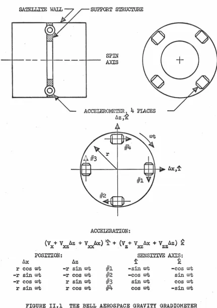
Bell Aerospace of Buffalo, New York, and Hughes Research of Malibu, California. The Bell Aerospace design calls for four directional

accelerometers rigidly attached to the walls of a cylindrical, spin stabilized satellite. The sensitive axis of each accelerometer would be directed tangentially, i.e. the proof masses inside the accelero-meters would be constrained radially. The signal from diagonally opposing accelerometers would be added and the pair of resulting

signals would be subtracted~ The Bell Aerospace accelerometers have been flight qualified and used in several satellite programs in other configurations.

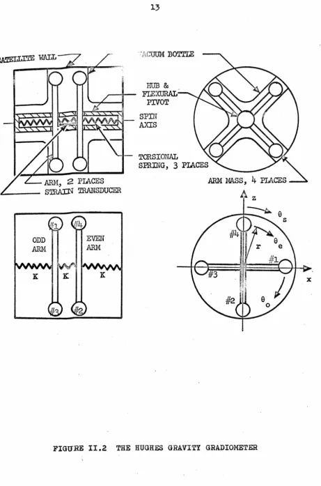
The Hughes design calls for a pair of torsional spring-mass oscillators, composed of two arms in the shape of a cross, with

torsional springs cross connecting the arms and connecting the arms to the walls of a spin stabilized satellite. Heavy proof masses would be located on the ends of the arms and the "difference" mode of the

II. 1 Gradiometers Constructed .from Accelerometers

Taking the proposals one at a time, consider the Bell Aerospace

instrument operating at a fixed point in a gravitational field which

varies slowly with position. The situation is indicated in Figure II. 1.

Think of an accelerometer as a proof mass sliding on a frictionless

wire. The proof mass is centered electronically so that a signal is

produced which is proportional to the force required to maintain the

proof mass at the center of the wire. Thus the signal is proportional

to. the acceleration relative to the accelerometer housing that the proof

mass would experience if free to travel along the sensitive axis. The

entire system rotates about the y axiso The acceleration due to this

rotation is radial and the sensitive axes are tangential; thus no signal

is produced by the satellite rotation.

The situation due to the gravitational field is different,

how-ever. Since the field is slowly varying, one is justified in writing a

Taylor's series expansion for the gravitational potential. This must

be carried to at least second ordero By differentiating the Taylor's

series expansion with respect to each of the coordinate axes one

obtains the vector acceleration of the proof masses as a function of

position (x, y, z)o Substituting expressions for sinusoidal motion in

the x, z-plane as a function of time, and dotting these expressions with

a time variant unit vector in the direction of each accelerometer's

sensitive axis (i.e., taking the vector component of acceleration in

the direction of the sensitive axis), one obtains the four equations

10

SUPPORT STRUCTURE

SPJN

AXIS

ACCEIEROMETER A.

4

.

PIACES 6z)-.it

ACCEIERATION:

(V

+

V flz

+

V

Ax)

1-

+

(V

+

V flx

+

V /lz) ·~ x xz . xx . z xz· zz

POSITioN: SENSITIVE AXIS:

~ ~

t

~

r

cos

wt

-r

sin wt

-r

cos

wt

r sin wt

-r sin wt

-r

cos

wt

r

sin wt

r

cos

wt

#1

#2

#3

#4

-sin wt

-cos

.

wt

sin

wt

cos

wt

-cos

wt

sin

wt

cos

wt

-sin

wt

[image:20.615.110.541.83.692.2]

s

₁oc -sin wt V - cos _x wt V _z

+

r sin wt cos wt(V _{. zz} -V )- r(cos_xx 2 wt-sin2wt)V _xz

s

₂oc-cos wtV +sin wtV- r sin wt cos wt(V -V )+ r(cos2 wt-sin2wt)V

x z zz xx xz

s

₃ oc sin wt V

+ cos

wt

V + r sin wt cos wt(V -V )- r(cos2

wt-

sin2 wt)V

x z zz xx xz

s

₄ oc cos

wt

V - sin wt V - r sin

wt

cos wt(V -V )+ r(cos2 wt-sin2wt)V

x z zz xx xz

(II. 1)

The satellite response is just enough to cancel the first order

derivatives in equation II. l except for satellite drag terms. This is

the reason that the signals can not be combined to measure

acceler-ation. However, by adding the signals from diagonally opposing

accelerometers and subtracting the resulting pair of signals, one

obtains the signal equation for the Bell Aerospace gradiometer.

Signal oc sin 2

wt (

V - V ) - 2 cos 2 wt V

zz xx ' xz (II. 2)

Satellite drag can be measured using the same four

acceler-ometers in this configuration. This is done by subtracting opposing

pairs of signals and adding the resulting pair of signals. The

resulting signal has an amplitude proportional to the in-plane drag

12

II. 2 Mechanical Gradiometers

Next consider the Hughes instrument operating at a fixed point

in the same gravitational field. By balancing the moments of the

gradiometer arms1 one can show that the ideal equations of motion

for the simple three degree of freedom system shown in figure II. 2

are:

I

0

+

K ( 8 - 8 )

+

K ( 8 - 8 )

=

m r 2 { ( V - V ) sin 2 8 -2 V cos 2 8

0 }

o o e o o s . zz xx o xz

,,

- 8 )

=

-mr2{(V - V ) sin 28 -2V cos 28 l

s zz xx e xz ef

I 8

+

K( 8 - 8 )

+

K ( 8

e e o o e

"

I (J

+

K (2 8 - fJ - 8 )

=

Drag Torque

s s o s o e (II. 3)

Taking the sum and difference of the first two equations one

can very nearly separate the difference equation from the other two.

Define 8

=

B - 8 and 2 Ot

=

e

+

8 where (j is proportional to the

o e o e

strain measured by the Hughes instrument.,

,, 2

IO+ (2K - K )6

=

2mr

{CV -

V ) sin 28t - 2V cos 28tl cos8

o zz xx . xz

r

zret'

+

2K (8t - 8 ) = 2mr2

{(v -

V ) cos 28t

+

2V sin 2 (Jt } sin 8

0 s zz xx xz

II

I 8

+ 2K (

(J - 8t)

=

Drag Torque

s s 0 s (II. 4)

Since the difference between the arm deflections, 8, is very ·

small, the last two equations approach the solution: 8 s

=

.8t

=

wt.

'

SATELLITE

WALL

ARM,

2 PIACES

£----

STRA:cN TRANSDUCER

TORSI

ON

AL

SPRING,

3

PIACES

[image:23.623.106.568.58.755.2]

l'+

quantity w

=

(2K - K )/I, the resonance frequency of the sensor; and

g 0

after observing that I

=

2mr2; one obtains equation II. 5.

8"

+

- - £ WQfY 9'

+

W 2 8 -- ( V - V ) sin 2 wt ~ 2 V

. g zz xx xz cos 2wt (II. 5)

This is the classical harmonic oscillator with a periodic

forcing function. Hughes proposes to increase the amplitude of

0

by picking the stiffness of the torsional springs such that w

=

2w. g

Under this condition, the forcing function on the right is forcing the

system at resonance, thus the steady state solution to equation II. 5

is as shown belowe

Q

(J

= -

2 (2.w)

j (V - V ) cos 2wt

+ 2V

sin 2wt}

l zz

xx

xz (II. 6)

The output of the Hughes strain transducer is proportional to this

quantity, thus the Hughes output equation is the same as the

Bell Aerospace output equation except for a 90° phase shift.

II. 3 Observations about the Signal Equation

There are several points it is important to realize about the

gradiometer signal. Firsti one should realize that the instrument

measures a combination of second derivatives of the gravitational

potential. It is hoped in this way to extend the range of frequencies

that the instru.rnent can measure, and also it is possible to measure

this quantity directly in free-fall.

Second, the signal comes at twice spin frequency. This

allows separation of the actual signal from a number of noise

the derivation it should be clear that the instrument must be rotated to

produce a signal, thus a spin stabilized satellite is called for.

Third, the equation is an approximation based on the Taylor's

series expansion for the gravitational potential. This is a very good

approximation. There are two length scales for the potential: the

altitude of the satellite above the surface and the radial distance to the

center of the earth. The dimensions of the gradiometer are small

compared to either scale.

Fourth, as a consequence of the derivation, the expression

involves second derivatives with respect to a spacecraft defined local

Cartesian coordinate system. This is unfortunate as an earth centered

spherical coordinate system is more natural for gravitational work.

Finally, it is important to realize that both amplitude and

phase data are associated with the signal. The amplitude is given by

equation II. 7:

Amplitude oc ,./(V - V )2

+

4 V 2

" zz xx xz (II. 7)

and the phase angle is within an additive constant of equation II. 8.

Phase

=

tan -1

2V xz

v

- v

zz xx

(II. 8)

Both Hughes and Bell Aerospace derive this equation in different ways.

By way of comparison the reader could refer to the appropriate

16

II. 4 Error Sources in the Signal Equation

The signal equation is not exact. A number of hardware effects must be considered before one is justified in talking about the signal in this waye Some of the larger errors that must be considered are: 1) long term drifts of the instrument proportionality constant, 2) errors in the orientation of the satellite spin vector~ 3) orbital responses to the higher degree terms in the gravitational field, 4) finite spin rate effects, and 5) the instrument signal to noise ratio. These error sources will be discussed in detail in a subsequent chapter (Chapter V) and will only be described herea Another class of at least equally important error sources arises from misalignments of the instrument. These are not within the scope of this thesis ..

The signal equation, IL 2~ expresses a proportionality between the output signal and the gravitational fielde The accuracy of this relationship is limited by the accuracy to which the proportionality constant can be made to hold constant. A number of factors act to change the proportionality constant in orbit. The most important factor will probably be changes in temperature in the satellite. This problem is easily understood in the case of the Hughes instrument. The

strain transducer Hughes uses to obtain a readout is functionally dependent on the temperature.

The signal equation is dependent on the orientation of the satellite's spin vector (i.e., the orientation of the x, z-plane with

orientation of the spin vector needs to be accounted for in the data reduction. If changes in orientation smaller than the smallest angular position that can be determined caused output signals larger than the instrument significance level, the data could not be corrected. This happens in the case of the angular position with respect to the in-plane

rotation, thus the phase angle from equation II. 8 can not be measured as accurately as the amplitude can be measured.

The satellite responds to the higher harmonics in the earth's gravitational field. One of the reasons for measuring gravity in the first place is to facilitate prediction of this response, i.e., orbit determination. Obviously this effect must be taken into account in the data reduction procedureo If the error in predicting the response of the satellite were large enough to cause signals of the order of the instrument sensitivity, a simultaneous solution for the satellite

response and the gravitational field would be necessary to remove this effect.

The cause of finite spin rate errors can be seen most clearly by considering the differential equation for the Hughes instrument expressing the way the signal is transmitted thru the proof masses (equation II. 5 copied below).

fl 2w I 8

+-fJ

Q

2

+

4 w (}

= (

V - V ) sin 2 wt - 2 V cos 2 wt

xx xx xz

(II. 9)

Since the satellite translates, V - V and 2V can be expressed

zz xx xz

18

frequency of the forcing on the right. The product of the spin rate

term and any of the frequencies from the terms V - V and V

zz xx xz

is equal to a sum of sine waves at the sum and difference of the

frequencies. If the satellite spin rate, w, is essentially infinite with

respect to the highest frequency of interest there is no problemo For

a finite spin frequency the attenuation can be rather large.

The instrument signal to noise level is one of the limiting

factors in the design of a gravity gradiometer. Essentially, this

problem arises because of Brownian motion of the test masses. This

random vibration creates a signal which can not be distinguished from

the gradiometer signaL Electrical noise is also a factoro Hughes

develops an equation for the signal to noise ratio which can be found in

reference I 0.

Finally, the reader should be aware of the nature of the

mis-alignment problems mentioned earlier as being outside the scope of

this thesis. These occur because of assumptions made in the

deriva-tion of the signal equaderiva-tion that can not be met preciselyo For example,

it was stated in deriving the signal equation for the Bell Aerospace

gradiometer that the sensitive axes of the accelerometers were

oriented tangentially. This is not possible to arbitrary accuracy ..

Similarly, the geometric center of the two instruments were both

assumed to lie on the spin axis. Again this can not be done to arbitrary

accuracy.

Most of these error sources are intimately coupled to the

20

III. THE SIGNAL IN SPHERICAL HARMONICS

Equations will be developed for calculation of the gradiometer

signal from known spherical harmonic coefficients.

The spherical harmonic expansion for the earth's gravitational

field is derived by recognizing that the gravitational field satisfies

Laplace's equation in spherical coordinates. By applying separation of

variables and requiring continuity at the coordinate boundaries and a

zero potential at infinity, one arrives at equation III. 1 for the

gravi-tational field exterior to a sphere of radius R.

n GM

~

(Rr)n V(r,X,cl>)

= -

L

r

L

Pnm(sin cl>)[Cnm cosmX +Snmsin mX] n=o m=o

(III. 1)

The problem with using this representation of the earth's field to

rep-resent the output of a gravity gradiometer is that the expressions for

the second derivatives with respect to a Cartesian coordinate system

are extremely complicated. This is obvious when one considers the

chain rule expansion for the second derivative of a function 6£ three

variables.

2 \ 2 2

V

=

V r

+

V'\ A

+

V"" cJ> + V r + V'\ '\I\ + V,,,.,,,. cJ>

xx r xx " xx

'*'

xx rr x "" x

'*''*'

x

+

2(V \r A

+

V ""r <I>

+

V'\"'-X cl>)

r"' x·x r'*' x x "'*' x . x

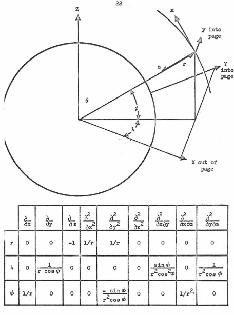
III. 1 Derivatives with Respect to Local Satellite Coordinates

By working at an arbitrary point in space and defining the local

x-axis in the direction of

¢,

the latitude; the local y-axis in the

direction of ,\, the longitude; and the local z-axis in the opposite

direction of r, the radius; all but two of the terms in equation III. 2

are identically zero. Figure III. l defines this coordinate system. It

is necessary to take first and second derivatives of the spherical

coordinates with respect to the local coordinates. This requires the

transformation between the two coordinate systems. The

transforma-tion between global coordinates and the local coordinate system is

indicated in equation III. 3.

X

=

cos A. sin<P x - sin X y +cos A cos <P(r z)

Y - - sin X sin cl> x

+

cos I\ y

+

sin ~ cos cf>( r z)

Z

=

cos cf> x

+

sin c;J>(r - z) (III. 3)

Working with equation !IL 3 and the transformation between

global and spherical coordinates, it can be shown that the derivatives

of the local coordinates with respect to the spherical coordinates are

as shown in Figure .III. L Substituting these expressions into the chain

rule expansions for the second derivates of equation III. 1 with respect

z

0

~

_{~ ~}

L

_ox

2

~

A

r 0 0 -1 l/r

'.

A

0 1 0 0 r cos

cp

¢

_l/r

_{0 0 0}

22

x

02

_?P

02

-

_dxoy

o:v2

_oz

2

l/r

0 0

0 0 sin <.2,

2

2

r cos

cp

- sin

cf>

_{0 0}

r 2 cos

¢

~

y into

page

y into

page

X

out of

page

2

fxaz

_fuz

2

0 0

0 ~ < 2 1

I

r

cos¢

l/r

21 0

[image:32.618.93.549.58.672.2]

00

I

n=o

. GM

V

(r,X,<P)=-3

yy r

00

I

n=o

GM 00

vzz(r,A,<P) = - 3

I

r n=o

GM 00

V (r,A,cj>)

=

-3

L

xy r _n.=o

GM 00

vxz(r,A,<I>) =-3

I

r n=o

GM 00

V (r,A,cP)

=

-3

L

yz r _n=o

n

~ pxx (sin 4')

re

cos mA

+

S sin m,\l

L... nm L nm nm ~

m=o

n

"' pYY (sin <P)

[c

cos mA

+

S sin m,\]

~nm nm nm

m=o

n n

(

~) ~

Pzz (sin <t>)

[c

cos m.A+ S sin mA]

r L.. nm nm nm

m=o

(R)n n

-_r "' pxy (sin <P)

[s

cos mA- C sin mA]

L.. nm nm nm

m=o

n n

(

~) ~

pxz (sincp)

[c

cos mX

+

S sin m,\]

r L... nm nm nm

m=o

(Rr)n

Ln

_{pYZ (sin<t>)[S cos mA - C sin mi\)}

nm nm nm

m=o ·

(III. 4)

Pxx (sin cl>)

=

nm

pYY (sin <J>)

=

nm

Pzz (sin ct>)

₌

nm

Pxy (sin cl>)

₌

nm

pxz (sin ct>)

₌

nm

pYZ (sin <i>)

₌

nm

24

d 2 P ( s in cl>) nm

- (n

+

1) P (sin <J>)

nm

~

+ (

n

+

1) p (sin <J>) - sin <J> nm (

2 ) d P (sin <J>)

cos2ct> nm cos<J> dct>

( n

+ 1 )( n

+ 2} P

( sin cl>) nm

m (sin

2"'

p nm (sin <J>)

+

1

d P (sin <J>)j

nm cos"' d(/) cos

q,

d P (sin <J>)

(n

+ 2)

nm d<J>

(III. 5)

m (n

+

2) Pnm (sin</>) cos"'

The equations have been written in this way to emphasize that

the form of the spherical harmonic expansion has been preserved.

There is a term containing the units, GM/ r ; a term expressing 3 . altitude variations, (R/r)n; a polynomial in latitude, P!!m(sin<P); and

sinusoidal variations in longitude, cos mX and sin mA. . From a dimensional argument one can see that the altitude variations must

take this form regardless of the orientation of the local coordinate

system. Since the local x direction is perpendicular to _the unit vector in the direction of A and the local y direction is

perpendic-ular to the unit vector in the direction of cb, it is obvious that the

III. 2 Evaluation of the Polynomials

By applying the chain rule expansion, one can show that the

polynomials from equation III. 5 may be written as shown in III. 6

below"

pxx (t)

nm

pYY (t)

nm

pXY (t) nm

pxz (t)

nm

2 d2Pnm(t)

=

(1 - t ) 2

dt

d p (t)

t nm

dt

(n

+

1) P (t)

nm

2 ) d p

(t)]

m 2

+

(n

+

1) p (t)

+

t nm

- t ) nm dt

=

m t p (t)

+

nm

(

d p

(t))

(1 - t2) nm dt

d p (t)

nm dt

pYZ (t)

=

m(n

+

2)(1 - t2

)

-

i

P (t)

nm nm

(III. 6)

The polynomials in equation III. 6 are always finite. This is

not obvious from the form in which they are written, but it follows

from substitution of Rodriques' formula for the associate Legendre

polynomial, equation III. 7.

p (t)

nm

=

dn+m (t2 _ l)n

26

Equation III. 4 satisfies Laplace's equation. The sum

pxx

+

pYY

+

pzz is zero since it is equal to the governing equation

nm nm nm

for the associated Legendre polynomialg equation III. 80

d ( 2 d p

(t)) (

dt ( 1 - t )

~~

+

.

n(n

+

I) - m2 ) p (t)

=

0

( 1 - t2) nm

(III. 8)

From this much information it is possible to calculate the

value of the second derivatives at any point using the recursion

formulas for the associated Legendre polynomial and the equations

just developed for the second derivatives. For example, using

Rodriques' formula it can be shown that the first derivative of the

associated Legendre polynomial with respect to t is given by

equation III.

9.

d p (t)

nm

dt

= -

n t P nm (t) .,_ (n

+

m) P n- ,m 1 (t)

(III. 9)

Substituting this expression into the governing equation one obtains a

three-term recursion relation for the associated Legendre polynomial.

(n - m

+

1) P

+

1 (t) = (Zn

+

1) t P (t) - (n

+

m) P 1 (t)

n , m n, m n- , m

This allows simple calculation of Legendre polynomials and

their fir st derivative. In order to start the procedure, one uses

Rodriques' formula to obtain an expression for the terms of equal

order and degree, i.e., m

=

n:

(2m)!

2m I

m.

(III. 11).

and the special cases PO,

0(t)

=

1 and P11 0(t)

=

t. Also from

Rodriques 1 _{formula it is clear that P (t)}

=

_{0 for m greater than n.}

nm

The reader should be warned that equation III. 10 is known as

an unstable recursion relation since the coefficient multiplying the

terms on the right is larger than unity. The argument here is that any

error in P _nm will be larger in P _n

+

_{1 ,m} due to being multiplied by a

number larger than one. If the reader is concerned about this, a

variety of other recursion relations are available ( 15).

III. 3 Relating the Second Derivatives to the Signal Equation

At this point it becomes necessary to relate the signal equation

(II. 2) to the expressions for the second derivatives (III. 4). This is

not as straightforward as it might appear since the orientation of the

coordinate system for the signal equation was fixed by the plane of the

gradiometer while the coordinate system for the second derivatives

was fixed by the location of the gradiometer. In general one of the

two coordinate systems must be rotated to the other.

The situation is further complicated by the requirement that

the satellite be spin stabilized to provide the necessary rotation for

28

space not in earth centered space. For normal usage of the

gradio-meter in a satellite, there is no problem. If the orbit is polar to

obtain complete coverage of the earth, and if the spin vector of the

satellite is perpendicular to the plane of the orbit, the derivatives of

Section IIL 2 can be substituted directly into the signal equation. If

either of these conditions are not met, the derivatives of Section III. 2

must be rotated to the coordinate system in which the gradiometer is

operating.,

In general an Euler angle transformation is required to

per-form the necessary rotation. First the rotation to inertial space is

required. This was already given as equation III. 3 repeated as a

matrix equation below.

(III. 12)

Where

[A

1

is:

- sin <f> cos )\ - sin X. - cos</> cosX. cos

x.

- sinX. 0 - sine/> 0 - cos </>

- sin<:fa sin A. cos

x.

- coscp sinX.

=

sinX. cos

x.

0 0 1 0

cos¢ 0 -sin¢ 0 0 I cos<f' 0 - sin</'·

This may be viewed as a rotation of </>

+

90° about the local y-axis

followed by a rotation of -X. about the global z-axis. The

transfor-mation from global to local coordinates is the transpose of this.

Having rotated to global coordinates, the next step is to orient

the satellite in the plane of its orbit. To do this the more general

I

LINE OF

I

APSIDES

I

f

NORTH

SATELLITE

.OB.BU,.

j.__.

---

--....;

/

-- -

A

w--...,.

EQUATOR ~,

'

_'

'

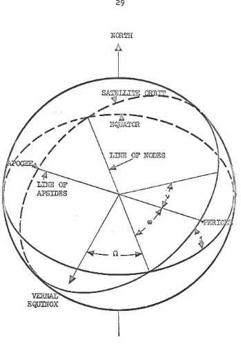
[image:39.620.153.502.57.555.2]

30

right ascension of the node; i, the orbit inclination; w, the argument

of perigee; and v, the. true anomaly. This coordinate system ·is

defined in Figure III.2. In general, to orient the y-axis (spin axis)

perpendicular to the plane of the orbit, the x-axis in the direction of

travel, and the z-axis downward in the radial direction, the

transfer-mation defined by equation III. 13 is required.

l

xsatellitel =

[BJ

l

xglobal

l

(III. 13) Where

[Bl

is:

- sin(w + v) 0 cos(w+v) I 0 0 cos

n

sin

u

0

0 1 0 0 sin i cos i -sin

n

cosn 0

-cos(Ci>+v) 0 - sin(w +ii) 0 -cos i sin i 0 0 1

Thus this transformation may be viewed as a rotation of

n

about the

global z-axis, followed by a rotation of (90° - i) about the new x-axis,

followed by a rotation of - ( (w

+

v)

+

9

o

0) about the new y-axis. This is

not a standard Euler angle transformation. Normally one rotates

about the z-axis, then the x-axis, and then the z-axis again(l6). This

series of rotations was used to allow the y-axis to be the spin axis

instead of the z-axis. Thus the total rotation for the second

deriva-tives is given by equation III. 14 ..

[

v.~atellite

J

Substituting 0 for w, </> for v, 90° for i, and ~ for

n,

one

discovers the transformation is unityo Thus, if a circular polar orbit

is used no transformation is required. This of course is what prompted

the selection of the coordinate system shown in Figure III. I in the first

place~

In the preceding transformations it was assumed that the spin

vector would be perpendicular to the plane of the orbit. This is not an

arbitrary choice. Another alignment would cause the large mean

signal to be modulated with the period of the satellite rotation about

the earth. This would create several problems. First, the character

of the signal would change during different parts of the orbiL At

worst the signal would change from small amplitude rather random

variations to large amplitude sinusoidal oscillations. The data

sub-system would need to be able to handle both cases. Further, phase

references would present difficulties. If the spin vector were in the

plane of the orbit, the satellite would have to shift between an inertial

and an earth centered phase reference to obtain orientation

informa-tion·. Finally, the signal would not be as nearly linear in terms of

the harmonic coefficients in any other orientation. Thus there ar~

hardware limitations and data reduction advantages that dictate this

32:

IV. AN INTEGRAL CURVEFIT TECHNIQUE

In this section an integral procedure will be developed for curvefitting the spherical harmonic coefficients of the earth's gravitational field. The procedure under consideration essentially involves a free air reduction of the gradient signal onto the surface of a sphere.. This corrected data can be integrated using theoretically derived weighting functions to orthogonalize the data. In order to evaluate the necessary integrals, the signal equation polynomials from equation III. 5 will be expanded in Fourier series. This raises the possibility of performing most of the calculations using a fast Fourier transform, thus reducing computer run time.

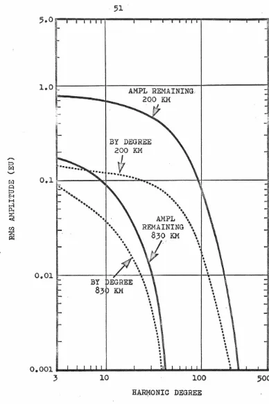
In proceeding in this way, the data reduction procedure is more like surface data reduction techniques than satellite data reduction techniques. This is made possible because the gradiometer signal amplitude is only a function of position and does not involve initial conditions. The gradiometer satellite is the only gravimetry

satellite proposed to date that has this characteristic. The prospects for actually making an integral procedure work are greatly enhanced by the effect of the satellite altitude. Since the satellite is flying well above the surface of the earth, the spherical harmonic expansion is highly convergent at wave lengths shorter than the satellite altitude. Further, global data will be available with the gradiometer satellite. Both of these advantages are not shared by existing surface techniques.

the higher harmonics is very much like the error in ground based data reduction introduced by not knowing the geoid height. At

satellite altitudes this error is considerably reduced for the higher harmonics by the attenuation of the response with altitude. Since the gradiometer measures a higher derivative than the satellite displace-ment responds to, it is reasonable that a data reduction procedure of this sort will converge at least as fast as surface data reduction procedures based on measuring acceleration.

IV. 1 Linearization of the Signal Amplitude

Since the phase angle of the gradiometer signal can not be measured to the accuracy that the amplitude can be measured, one is

constrained to fit data knowing only the signal amplitudeo The equa-tion for the signal amplitude is not linear (eq .. II. 7 repeated below). This difficulty can be overcome by

Amplitude oc

'1

(V - V )2

+

4 V 2

zz xx xz (IV. I)

recognizing that the signal from the mean earth (C ) very much 0, 0

dominates the signal. Expanding the signal amplitude equation according to the binomial theorem, one obtains equation IV. 2.

2

v

2

zv

4 Amplitude ~ (V - V )

+

xz

zz xx V -V zz xx

xz

+

(V - V

)j.

zz xx

TABLE IV.1 COMPONENTS OF THE GRADIOMETER SIGNAL

COMPONENT

TERM

EXPRESSION

C )

v

3

co,o

=

1

v

_zz

_xx

3

GM/r CO,O

2

v

0

xz

J2

=

0.001083

v - v

_zz

_xx

GM (R)

2

(57

15)

r3

r

4

cos

2(J +

4

J2

2

v

:~

_m2

12 sin

2(}

_J2

xz

n

~3

v

-

GM

_~

((Rt

_{r (n+l)(n+2)}

(10-5)

7

)2

_(2n+l)

•

zz

_r3

see ref.

9

AMPLITUDE AT

100 KM

4400 EU

0 EU

28

EU

18.5

EU

0.73 EU RMS

[image:44.793.127.682.187.428.2]

+-5000

4000

3000

2000

40

30

20

10

5

1

o.

5

o.

1

.id

MEA

~ SIGN

~L

"""

---.

...

----

_{____...}

----

-

~---ft - - - i - - . . . _

r,

r,

-.

~

vzz

.. v

xx

"'2

.

J2 /

/

-~

~

vxz

-\

\

\

·' "

"

_'

~

..

I"

'

_"

[

~

}'

_~

RMS

RAD I Al

SECOND

~

~

DER!\

ATIVE

~

...__

0

1 0

0

200

300

400

500

600

700

800

9l

0 lUOC

SATELLITE ALTITUDE (KM)

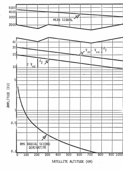
[image:45.618.122.550.80.671.2]

36

Figure IV. I is a plot of these results as a function of altitude. Using

these results one can further simplify equation IV. 2. Taking a

nominal altitude of 100 km one expects V - V to have a mean zz xx

signal larger than 4000 EU ( l EU

=

10-9 / sec2). The ellipsoidal bulge will contribute less than 30 EU to V - V i and there will be a

zz xx

perturbation signal of about 2 EU RMS. On the other hand, there is

no mean contribution to V so the ellipsoidal bulge dominates that XZ

term with a signal of the order of 20 EU. Again, the perturbation

signal to V will be relatively small, of the order of 1 to 2 EU RMS. xz

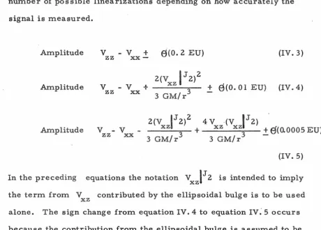
Substituting these results into equation IV. 2, there are a

number of possible linearizations depending on how accurately the

signal is measured.

Amplitude V _zz - V _xx-

+

0(0. 2 EU) (IV. 3)

Amplitude

2(V

I

J 2)2

V - V

+

xz

+

8(0. 0 I EU) (IV. 4) zz xx 3 GM/r3

Amplitude

v - v

zz xx

2(V IJ2)2 4V ·(V

IJ2)

xz .

+

xz XZ

+

EJ(0.0005 EU) 3 GM/r3 3 GM/r3

(IV. 5)

In the preceding equations the notation V

IJ

2 is intended to imply xz

the term from V contributed by the ellipsoidal bulge is to be used xz

alone. The sign change from equation IV. 4 to equation IV~ 5 occurs because the contribution from the ellipsoidal bulge is assumed to be

[image:46.615.95.556.344.674.2]

Another linearization procedure is perhaps easier if one

considers using the data from a gravity gradiometer to improve the

values of an existing reference field. Under this condition one would

be able to form an estimate of the amplitude from the reference field

using the actual signal amplitude equation (IV. .. 1) o If one subtracted

the value of V - V calculated from the reference field from the

zz xx

amplitude calculated from the reference field, the result would be the

correction to the actual signal to linearize it so that equation IV. 3

held. This has the advantage that the correction is expressed totally

in terms of the reference field. Algebraically equation !Vo 6

illus-trates this procedure~

(IV. 6)

This procedure will have an error of about four times the error in

predicting V in the reference field times the value of V

xz xz

contributed by the ellipsoidal bulge divided by the mean signal

amplitude. In any event$ this procedure is more accurate than the

one implied by equation IV. 4 as long as the reference field is at least

as complicated as the reference ellipsoid. This linearization

procedure was the one used in subsequent calculations.

IV. 2 Derivation of Integral Curvefit Technique

One starts to develop the integral curvefit equations by writing

down the signal equation and identifying the signal as the actual

38

V V = Signal

zz xx

GM

3 " R

~

G (<f>)(C cosmA+S mA)=Signal(r,Alt>)

oo

(~n

n

L.J r nm nm

nm

r n=o m=o

G (cp) = pzz _ pxx

nm nm nm (IV. 7)

Multiplying on both sides by G .. (<I>) cos j,\, requiring r to be constant11

lJ

and integrating over a sphere of radiusp r, one obtains equation IV. 8.

1

f

211" 2ir oo n oo

GM₃

f

L

~~)

L

G (<l>\G .. (cp)(C cos

mA

+S sin m,\)

r nm<1J nm nm

r n=o m=o

1 0

-zrr

2ir

Signal G .. (<;i>) cos jA co

scp

r2

cL\

dcp

lJ

(IV. 8)

Next one formally interchanges the order of integration and .summation.

Since sines and cosines are orthogonal one can drop the summation

over m~ replace m by j, and integrate with respect to ,\.

C .

J

trr

G {</>)G •. (</>) cos</> d</>

nJ nm lJ

. 1

-zrr

(IV. 9)

J

-}IT!

Zir

= Signal G .. (sf>) cos

j~

coscp r2dA dcp

lJ

1

Realizing that the integral remaining on the left side is just a

number, what is left is an equation relating the coefficients of the

theoretical expansion to the actual signal. This is the C .. -th

lJ

equation. Replacing the cos jA by a sin jA and repeating the process,

one can obtain a similar S .. -th equation. Conceptually, repeating the

lJ

process over all i and j one has an equation for each coefficient.

and where:

c ..

JJ

s ..

JJ

0 .. nJl

s

I..

lJ

0 ...

JJl

0 ...

JJl

+ ....

+

s .

nJ

0 ..

llJl

0 ..

IlJl

+ •••

+

0 • 0

c

=I..

lJ

s

=

I..

lJ

=

rr r2

~ (~)nf

-}rr

G

.(</J)

G

..

(</') cos</J

:J r nJ lJ

r i

dcp

- 211"

f

-}rrf

2rr

=

1

Signal (r~,\ ,'f>)Gij(</') cos jA

-211" 0 .

2

cos</' r dA d</'

2

coscpr_

dA

dcp

(IV.IO)

A word on notation is in order here. The use of three indices

instead of four in the previous equation is confusing. The notation

0 . . is intended to imply the coefficient relating the C . harmonic

~1 ~

to the C.. harmonic is being worked with. The coefficients relating

lJ

the C harmonic to the C.. harmonic for m =/:. j are all zero.

nm lJ

40

found to be zero due to orthogonality in equation IV.

9.

The resulting

matrix of coefficients is indicated in Figure IV. 2 for a system

truncated at n = 5. It will be shown in the next section that only

coefficients of the same parity in n and i (i. eo, n even and i even

or n odd and i odd) are non zerov This accounts for the arrangement

of the variables.

At this point one is dealing with a matrix composed only of

theoretical quantities on the left and a fairly complicated column

vector of integrals of the real signal (mapped on a sphere) on the right.

The system looks as follows:

f

o ..

J

{c . }

L

nJi nJ

=

{I~.

lJ

}

ro ..

J

{s . }

l

nJl nJ

=

h~.}

lJ

(IV. 11)

If the system is non-singular, it can be solved for the coefficients by

inverting the observation matrix and multiplying on the right.

Ex:peri-mentally the author has shown the system is non singular, i.e., each

non-zero partition has a finite determinant which can be made as large

as desired by scaling. Further, the size of matrix that needs to be

inverted is small~ Inverting by partitions» the largest matrix that needs to be inverted has a dimension of about n/2. Since the system

converges, i.e., the integrals on the right become negligibly small,

the infinite system of equations developed here can be truncated at

wave lengths about equal to the altitude the satellite flies at. This is

n

n

m

0 0

2

·

0

4

0 1 0 J ·O 5 0 1 1 3 1

5 1

2

1

4

1 2

2

4 2

3 2 5 2

3 3 5 3 4 3

4 4

5

4

5

5

0 2 4

1 3 5 1 3 5

2 4

2 4

3 5

3 5 4 4 !=) ₅

0 .. 0 0 0 0 0 1 1 1 1 1

2 2 2 2

3 3 3

4 4

5

x x x

x x x

x x x

x x x

x x x

x x x

x x x

x x x

x x x

x x

x x

x x

x x

x x

x x

x x

x x

x

x

x

x

x signifies a non-zero number

FIGURE IV.

-

2

FORM OF THE OBSERVATION

MATRIX

[image:51.620.139.423.97.387.2]

42

IV. 3 Expansion of Polynomials in Fourier Series

The construction of the observation matrix requires expansion

of the theoretical integrals from eq':lation IV. 10. This is readily

. accomplished if one observes that the polynomials have a simple

expansion in terms of a Fourier series. Returning to equation III. 5

one discovers that the polynomials may be represented as shown in

equation IV. 120

d2P (sin¢ )

G ( ¢) = P z z - Pxx = ( n + 1)(n+3) P (sin

cp ) -

nm

nm nm mn nm d¢2

(IV. 12)

The associated Legendre polynomials have a Fourier series

I

which terminates with the term ncpc Further» if one converts to

colatitude, (}, instead of latitude,

<P,

(where 8

=

'TT - ¢) the Fourier

series expansions have the properties shown in .Table IV .. 2.

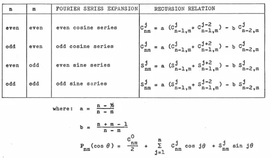
The coefficients of the Fourier series expansion are readily

calculated from the recursion relations discussed in Section III. 2

by calculating a new recursion relation for the coefficients of the

Fourier series expansion. This is done by substituting the Fourier

series expansion into the recursion relation and equating amplitudes

of frequencies.. The results of this operation are shown in Table IV. 2

for the recursion relation indicated in equation III. 10.

The procedure may be started by the use of the formula

n

m

even even

odd even

even odd

odd odd

FOURIER SERIES EXPANSION

even cosine series

odd cosine series

even sine series

odd sine series

where: _a

=

n - ~ n - m

b =

n

+

m -

l

n - m

co

P (cos8)

=

nm 2

nm

RECURSION RELATION

cj

=

a (cj + cj-2 ) - b cj nm n-1,m n-1,m n-2,m

cj

=

a (cj + cj+2 ) - b cj run n-1,m n-1,m n-2,m

sj = a (sj + sj+2 ) - b sj nm n-1,m .n-1,m n-2,m

sj = a (sj + sj-2 ) - b sj nm n-1,m n-1,m n-2,m

n

cj cos j8 + sj sin j8

I

+

j=l

nm nm

+-"

[image:53.799.148.685.161.474.2]