From PID to L1 Adaptive Control for Automatic Balancing of a Spacecraft Three-axis Simulator

(1)

International Journal of Emerging Technology and Advanced Engineering

Website: www.ijetae.com (ISSN 2250-2459, ISO 9001:2008 Certified Journal, Volume 6, Issue 1, January 2016)

77

From PID to L1 Adaptive Control for Automatic Balancing of a

Spacecraft Three-axis Simulator

Hung Truong Xuan

1

_{, Ahmed Chemori}

2

_{, Tuan Pham Anh}

3

_{, Huy Le Xuan}

4

_{, Thu Phan Hoai}

5

_{, Phuong Vu Viet}

6

1,3,4_{University of Science and Technology of Hanoi; 18, Hoang Quoc Viet street, Cau Giay, Hanoi, Vietnam} 2_{The Montpellier Laboratory of Informatics, Robotics and Microelectronics; UMR 5506 - CC 477 161 rue Ada, 34095}

Montpellier Cedex 5, France

1,3,4,5,6_{Vietnam National Satellite Center, Vietnam Academy of Science and Technology; 18, Hoang Quoc Viet street, Cau Giay,}

Hanoi, Vietnam

Abstract— Spacecraft three-axis simulators consist mainly in weightless and, ideally, frictionless hardware platforms. They are inevitable for validation of spacecraft attitude determination and control strategies and their associated testbed has to warrant firmly its weightless state during operation by using the automatic balancing mechanism. This paper proposes two different control schemes for the mechanism to ensure the weightless state. They are cascade PID control system and L1 adaptive control (L1-AC) system. Some different simulation scenarios are considered to analyse the effectiveness and performances of the proposed control solutions.

Keywords— automatic balancing system, L1 adaptive control scheme, spacecraft three-axis simulators

I. INTRODUCTION

Satellite attitude determination and control strategies (ADCS) have a very important role and can affect crucially the satellite operation in orbit, especially for earth observation satellites. The functional test of that system is an essential part of the ADCS research and development (R&D) process. Several ADCS simulators have been developed and spherical air bearings have been used for nearly 45 years [1]. Although the air bearing can’t provide a micro-gravity state, it offers a nearly frictionless and weightless environment, mainly as close as possible to space, to allow its payload have simultaneously unconstrained angular motion in three axes. It can be a very suitable tool for ground-based research in spacecraft dynamics and control, such as attitude determination and control. The table-top rotation system is flavor type and involves both hardware integration and software development for many simulators.

FIGURE1:THE NAVAL POSTGRADUATE SCHOOL'S THREE AXIS

ATTITUDE DYNAMICS AND CONTROL SIMULATOR

(2)

International Journal of Emerging Technology and Advanced Engineering

78

CubeTas [5] was a compact simulator for Cube-sat scale and can balance automatically with sliding masses only. FACE is a spherical air bearing with satellite component platform, preliminary solar simulator, and magnetic field simulator [6]. FACE is also implemented automatic calibration software to adjust center of gravity (CG) point of the platform.

Besides, some control schemes have been proposed for balancing purpose of the testbed. For instance, the vector from the center of rotation (CR) to the CG was estimated by analyzing the dynamical data given by the rate and position sensors [7]. As a result, the testbed is able to balance within 10 minutes and the error between CG and CR was less than two hundredths of a millimeter. Some advanced schemes are proposed, such as adaptive control in [8], [9], adaptive control using three sliding mass only in [10]. All of them focus on automatic balancing task that improves performance and effectiveness and use a set of sliding masses as the main actuators. The control scheme, as derived in [9], also used additional desired spacecraft momentum trajectory that acts as constant maneuvering of the testbed, it was able to balance simultaneously in three directions. The adaptive control solution [10] could only balance the X, Y offsets between CG and CR. In order to compensate the Z offset, the unscented Kalman filter (UKF) was used to estimate the Z offset. There are also other proposed solutions for the balancing mission. For instance, a compensating method is proposed to overcome the unbalance torque results platform deforming of the air-bearing spacecraft simulator [17]. As description in [18], they propose sinusoidal strategy control to perform a platform rotation maneuver or a discontinuous time-invariant feedback controller is deduced using two proof mass devices [19].

II. MODELING OF AUTOMATIC BALANCING SYSTEM A. Introduction of the simulator

Vietnam National Satellite Center (VNSC) is developing a simulator for attitude determination and control of micro-satellite class as illustrated in Figure 2. It can simulate weightless, frictionless state, the Earth's magnetic field, and the Sun’s light direction. The most important component of this simulator is a testbed integrated with a spherical air bearing. It includes also several sensors (gyroscope, sun sensor, IMU and vision), a set of rough sliding masses and a set of fine sliding masses. Its operation can support automatic balancing solution.

FIGURE2:CADVIEW OF THE SIMULATOR DEVELOPED BY VNSC

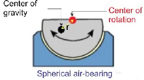
There are two coordinate systems to assign on the simulator, the first one is an inertial coordinate type named fixed frame coordinate system (-f), and the second one is a rotating coordinate type named testbed coordinate system (-t). Both of their origin coincides with the testbed center of gravity as illustrated in Figure 4. The weightless state can be derived from equilibrium state of the testbed, whose center of gravity coincides with the center of rotation as in Figure 3. Therefore, the testbed movement is no longer influenced by the Earth gravity and only the spacecraft ADCS operation affects it.

FIGURE3:SPHERICAL AIR BEARING AND BALANCING CONCEPT

The balancing mechanism is a sequence corresponding to two integrated sets of sliding masses. The rough ones are used firstly to redistribute manually the testbed mass/inertia moment. After that, the fine sliding masses are controlled automatically to achieve completely testbed weightless state. This automatically balancing phase has two stages including

[image:2.612.369.507.135.320.2] [image:2.612.372.514.472.551.2]

(3)

International Journal of Emerging Technology and Advanced Engineering

79

• Stage two: It is must be sure that if the testbed at equilibrium state, it will stand still or keep moving continuously at a constant speed. Hence the control idea is to change automatically positions of the fine sliding masses so that the testbed is able to move with constant velocity.

FIGURE4:ILLUSTRATION OF TESTBED (-T) AND FIXED FRAME (-F)

COORDINATE

B. Modeling of automatic balancing system

Because of momentum conservation law, the modified testbed dynamic equation can be derived easily in -t coordinate system [9]:

Where m is the testbed mass; Jt is inertial moment

matrix of the testbed, t is testbed angular rate, rt is

displacement between CG and CR of testbed, gt is the Earth

gravity. All of them are in -t coordinate. We assume that

And we also have

Where gf is the gravity vector in -f coordinate and Rft is

rotational matrix from -f to -t coordinate. Equation (1) can be rewritten as follows

Where Mt and Gt are defined matrix below

There is a strict relationship between the rotational testbed speed and the displacement from CR to CG in (4).

Because the testbed is also integrated a set of fine sliding masses, we are able to consider vector u to represent u = d1u1 + d2u2 + d3u3

where u1, u2, u3 are unit vectors of Oxt, Oyt, Ozt.

Combination of (4) and (7) is the final dynamic equation of the testbed, which is integrated a set of sliding masses, as shown following

where rt0 is intial position of rt and msl is the mass of the

sliding mass.

III. PROPOSED CONTROL SOLUTIONS

The proposed control solutions have to deal with the fact that displacement vector between CR and CG isn’t directly measurable. There are some other conditions to determine exactly when the CG-CR coincidence happens as already mentioned in previous section: the testbed should be on horizontal plane when balanced in X and Y axes; and it kept moving at a constant speed when balanced finally in Z axis. Two proposed control solutions are PID control and L1 adaptive control.

(4)

International Journal of Emerging Technology and Advanced Engineering

80

L1-AC can be considered as a modified Model Reference Adaptive Control (MRAC) scheme because its basic architecture is made from the internal model principle. The L1-AC can achieve high adaptation rates in conjunction with warrant the small error norms. It also integrates a low-pass filter on the control input to reduce significantly the high frequencies in the control signals and to be able to shape the nominal response.

A. PID control solution

This PID control scheme has a cascade structure as shown in Figure 5. Their parameters are determined firstly based on Ziegler - Nichols method, and then they are adjusted with a fine tuning.

FIGURE5:PIDCASCADE CONTROL SYSTEM

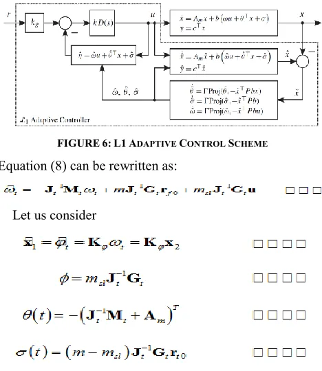
B. L1 adaptive control solution

Figure 6 illustrates the structure of the L1-AC scheme for a system with the presence of matched uncertainties. Am, b and c are well-defined matrices [12].

FIGURE6:L1ADAPTIVE CONTROL SCHEME

Equation (8) can be rewritten as:

Let us consider

Where K is conversion matrix; Am is desired Hurwitz

matrix. Then we will have:

where Bm and Cm are well defined matrices.

We also have , ,  are unknown nonlinear parameters and need to be estimated. Since all parameters: m, msl, Rft,

Jt, rt0 are bounded or well known then we can assure that , ,  are bounded easily:   = [l0 h0];   = [l0

h0]; [l0 h0].

Consider the following state predictor now

With

Are estimation of x2, , , . If we assume the error of

the state estimation is

!

x

2

=

⌢

x

2

-

x

2

Then we can propose the following adaptation laws with the projections

Where  is adaptation gain; P = PT_{> 0 and it is the}

solution of the following algebraic Lyapunov equation

for any arbitrary matrix Q, such that Q = QT > 0. Because , , are already bounded, the equations (17) will be bounded too.

According to Figure 6, the control signal is calculated by equation

[image:4.612.53.286.302.356.2] [image:4.612.50.284.431.701.2]

(5)

International Journal of Emerging Technology and Advanced Engineering

81

D(s) is a feedback gain and a strictly proper filter leading to a strictly proper closed-loop system

With DC gain C(0) = 1. Otherwise, D(s) are also subject to the following stability condition

G

( )

s _L₁L<1

where

and

Equations (14), (15), (17), and (19) are design part of the L1 adaptive controller and the system will be bounded at the infinite time [12].

IV. RESULTS AND ANALYSIS

The SIMULINK simulation model are built based on these equations (8), (14), (15), (17), and (19). Due to the limitation of the real platform, we implement bounded conditions derived from testbed paramaters:

1,2[-35 35]; 3R (deg) m[10 40] (kg)

rt(X,Y)[-0.19 0.19] (mm)

d [-150 150] (mm)

and the dynamic parameters of system are the following:

m = 35 kg

Jt = [1.445 0.068 0.218;0.068 2.43 -0.068;0.218 -

0.068 1.445] (kgm2₎ msl = 0.2 kg

rt0 = [0.15;-0.15;-0.3] (mm)

d0 = [0;0;0] (mm) t0 = [0;0;0] (deg/s)

We choose these parameters for the L1-AC model Am = [-1 0 0;0 0 1;0 -1 -1.4];

Bm = [1 0 0;0 1 0;0 0 1];

Cm = [1 0 0;0 1 0;0 0 1];  = 100000;

and transfer matrix of the filters for control inputs are

D

( )

s = 1

s2₊_1.85_s₊₁

(

)

;

(

s2₊_1.851 _s₊₁

)

; 1

s2₊_1.85_s₊₁

(

)

é ë ê ê ù û ú ú

In order to analyze the effectiveness and performances of the proposed control solutions, different simulation scenarios are considered, including:

 Scenario 1: the nominal operation;

 Scenario 2: robustness test towards parametric

uncertainties, for instance a change in m and Jt;  Scenario 3: external disturbances rejections, such as

the disturbance leaded to a change in CG position and external moment impacted in certain time.

Simulation results will be analyzed then to understand the effective performance of two control schemes in automatic balancing system of the testbed.

A. Scenario 1: nominal operation

We simulate two proposed control schemes: PID and the L1-AC with the same set of parameters. Both control schemes were able to keep moving CG to CR after a certain time. These obtained simulation results of both control schemes are depicted in Figure 7 to 10. According to them, it can be observed some ripples in the curves of PID simulation while the L1-AC responses are very smooth, as shown in Figure 7. Figure 8 demonstrates testbed attitude and it is easily to see that the angular rate along Z-axis of the PID simulation is also quite larger than the one of the L1-AC simulation. Generally, the L1-AC control scheme performance is better than the PID one in this scenario.

A further analysises for the L1-AC scheme are already done. The estimation error is really small and is about 0,1% of testbed speed, as seen in Figure 9. It means the operation of state predictor, as illustrated in equation (15), is very good. Besides, figure 10 indicates that all the adaptation laws are clearly bounded as expectation during their evolution versus time. The L1-AC scheme design works very well with the testbed model.

B. Scenario 2: robustness test towards uncertainties

This scenario includes the following cases:

 Case 1: m = 30(kg); Jt=[1.267 0.068 0.218;0.068 2.13

(6)

International Journal of Emerging Technology and Advanced Engineering

82

 Case 2: m = 35(kg); Jt=[1.445 0.068 0.218;0.068 2.43

-0.068;0.218 -0.068 1.445](kgm2_);

 Case 3: m = 40(kg); Jt=[1.647 0.068 0.218;0.068 2.77

-0.068;0.218 -0.068 1.647](kgm2_).

The scenario results are illustrated in Figure 11 and the Table 1 summarizes performance characteristics of two control schemes, such as steady state error and settling time. According to these obtained results, we can easilly find out that the L1AC performance is more robust than PID one in this scenario.

TABLEI

PERFORMANCE OF ROBUSTNESS TEST SCENARIO

Mass (kg)

Steady state error Settling time (s)

PID L1AC PID L1AC

30 35 40 10% 1% unstable

1% (z: 1.3%) 1% (z: 1.3%) 1% (z: 1.3%)

300 220 unstable 300 220 200

C. Scenario 3: external disturbance rejection

Let us consider two cases of disturbance rejection. The first one is performed with assumption that CG position will be moved accidentally out of desired location, including three cases:

 Case 1: CG offset is [-0.05;0.05;0] mm;

 Case 2: CG offset is [-0.1;0.1;0] mm;

 Case 3: CG offset is [-0.2;0.2;0] mm.

TABLEII

PERFORMANCE OF EXTERNAL DISTURBANCE REJECTION

(NON-RIGID SCENARIO)

Mass (kg)

PID L1AC PID L1AC

30 35 40 1.5% 1.5% 1.5%

1% (z: 1.3%) 1% (z: 1.3%) 1% (z: 1.3%)

50 60 70 20 20 20

Figure 12 displays the result curves of two proposed schemes and the control performance of both schemes are summarized in Table 2. By comparing these results, we can point out that the L1-AC disturbance rejection is better than the PID when CG position location varies.

The second case of external disturbance rejection is done with the assumption that the external moment impacts on the testbed at the time instant: 5 second. The following simulated cases are considered:

 Case 1, Timpacted=[0.005;0.005;0] N.m;  Case 2, Timpacted=[0.0075;0.0075;0] N.m;  Case 3, Timpacted=[0.01;0.01;0] N.m.

Figure 13 shows the obtained simulation results of two proposed control schemes and their control performance are summarized in Table 3 to compare their effectiveness. We can easily find out the disturbance rejection of the L1-AC is better than the PID in this case.

TABLEIII

PERFORMANCE OF EXTERNAL DISTURBANCE REJECTION

(EXTERNAL MOMENT IMPACTED)

Mass (kg)

PID L1AC PID L1AC

30 35 40 1.7% 1.7% 1.7%

1% (z: 1.3%) 1% (z: 1.3%) 1% (z: 1.3%)

50 50 50 50 50 50

V. CONCLUSIONS AND FUTURE WORK

[image:6.612.43.293.483.541.2]

(7)

International Journal of Emerging Technology and Advanced Engineering

83

FIGURE7:CG POSITION RESULTS OF AUTOMATIC BALANCING CONTROL SIMULATION –NOMINAL OPERATION

(LEFT:USING PIDCONTROLLERS,RIGHT:USING L1ADAPTIVE CONTROLLER)

FIGURE8:TESTBED ATTITUDE OF AUTOMATIC BALANCING CONTROL SIMULATION –NOMINAL OPERATION

(LEFT:USING PIDCONTROLLERS,RIGHT:USING L1ADAPTIVE CONTROLLER)

(8)

International Journal of Emerging Technology and Advanced Engineering

84

FIGURE10:ADAPTION LAW ESTIMATIONS OF L1ADAPTIVE CONTROL SIMULATION –NOMINAL OPERATION

(LEFT:ΦESTIMATIONS;MIDDLE:ΘESTIMATIONS;RIGHT:  ESTIMATIONS)

FIGURE11:CGPOSITION RESULTS OF AUTOMATIC BALANCING CONTROL SIMULATION –ROBUSTNESS TOWARD UNCERTAINTY

(9)

International Journal of Emerging Technology and Advanced Engineering

85

FIGURE12:CGPOSITION RESULTS OF AUTOMATIC BALANCING CONTROL SIMULATION-EXTERNAL DISTURBANCE REJECTION/NON-RIGID TESTBED

(TOP:USING PIDCONTROLLERS,BOTTOM:USING L1ADAPTIVE CONTROLLER; FROM LEFT TO RIGHT IS X,Y,ZAXIS)

FIGURE13:CGPOSITION RESULTS OF AUTOMATIC BALANCING CONTROL SIMULATION-EXTERNAL DISTURBANCE REJECTION/EXTERNAL MOMENT

IMPACTED

(10)

International Journal of Emerging Technology and Advanced Engineering

86

Acknowledgements

This research is granted by the National Research Program for Space Science and Technology through the project ―Research and Development of a High Accurate Attitude Determination and Control System Simulator for Earth Observation Satellite - VT/CN-03/14-15‖.

REFERENCES

[1] J. L. Schwartz, M. A. Peckz and C. D. Hall, ―Historical Review of Air-Bearing Spacecraft Simulators", Journal of Guidance, Control, and Dynamics, Vol. 26, No. 4, pp. 513-522, 2003.

[2] C. O. Mittelsteadt and E. A. Mehiel, ―Cal Poly Spacecraft Attitude Dynamics Simulator: CP/SADS‖, AIAA Guidance, Navigation, and Control Conference and Exhibit, Hilton Head, South Carolina, paper No. 2007-6443, 2007.

[3] M. G. Spencer, V. Chernesky, J. Baker and M. Roman, ―Bifocal relay mirror experiments on the NPS three axis spacecraft simulator‖, AIAA Guidance, Navigation, and Control Conference and Exhibit, Monterey California, paper No. 2002-5031, 2002. [4] J. Prado, G. Bisiacchi, L. Reyes, E. Vicenta, F. Contreras, M.

Mesinas, and A. Juarez, ―Three-Axis Air-Bearing Based Platform for Small Satellite Attitude Determination and Control Simulation‖, Journal of Applied Research and Technology, Vol. 3, No. 3, pp. 222–237, 2005.

[5] H. Woo, O. R. Perez, S. Chesi and M. Romano, ―CubeSat Three Axis Simulator (CubeTAS)‖, AIAA Modeling and Simulation Technologies Conference, Portland, Oregon, paper No. 2011-6271, 2011.

[6] T. Kato, A. Heidecker, M. Dumke and S. Theil, ―Three-Axis Disturbance-Free Attitude Control Experiment Platform: FACE‖, Transactions of the Japan Society for Aeronautical and Space Sciences, Aerospace Technology Japan, Vol. 12, pp. Td_1-Td_6, 2014.

[7] Y. Li and Y. Gao, ―Equations of motion for the automatic balancing system of 3-DOF spacecraft attitude control simulator‖, International Symposium 3rd on Systems and Control in Aeronautics and Astronautics (ISSCAA), Harbin, pp. 248-251, 2010.

[8] J. J. Kim and Brij N. Agrawal, ―System identiﬁcation and automatic mass balancing of ground-based three-axis spacecraft simulator‖, AIAA Guidance, Navigation, and Control Conference and Exhibit, Keystone, Colorado, paper No. 2006-6595, 2006.

[9] J. J. Kim and Brij N. Agrawal, ―Automatic mass balancing of air-bearing-based three-axis rotational spacecraft simulator‖, Journal of Guidance, Control, and Dynamics, Vol. 32, No. 3, pp. 1005-1017, 2009.

[10] S. Chesi, Q. Gong, V. Pellegrini, R. Cristi and M. Romano, ―Automatic mass balancing of a spacecraft three-axis simulator: Analysis and experimentation‖, Journal of Guidance, Control, and Dynamics, Vol. 37, No. 1, pp. 197-206, 2014.

[11] J.L. Schwartz, and C.D. Hall, ―System Identification of a spherical air-bearing spacecraft simulator‖, Proceeding of AAS/AIAA Space Flight Mechanics Conference, Maui, Hawaii, paper No. 04-122, 2004.

[12] N. Hovakimyan, C. Cao, ―L1 Adaptive Control Theory Guaranteed Robustness with Fast Adaptation‖, Siam, US, 2010.

[13] S. Boyd and S.S. Sastry, ―Necessary and Sufficient Conditions for Parameter Convergence in Adaptive Control‖, Automatica, Vol. 22, No. 6, pp. 629-639, 1986.

[14] K. Nguyen and H. Dankowicz, ―Adaptive control of underactuated robots with unmodeled dynamics‖, Robotics and Autonomous Systems, Vol. 64, pp. 84–99, 2015.

[15] D. Maalouf, A. Chemori, V. Creuze, ―L1 Adaptive depth and pitch control of an underwater vehicle with real-time experiments‖, Ocean Engineering, Vol. 98, pp. 66–77, 2015.

[16] M. Bennehar, A. Chemori and F. Pierrot, "L1 Adaptive Control of Parallel Kinematic Manipulators: Design and Real-Time Experiments", IEEE ICRA'15, Washington, USA, 2015.

[17] Y. Li, G. Bao, and Z. Wang ―A New Method for the Compensation of Unbalance Torque of 3-DOF Spacecraft Attitude Control Simulator‖, International Symposium 1st on Systems and Control in Aeronautics and Astronautics (ISSCAA), Harbin, pp. 403-407, 2006. [18] Y. Li and Y. Gao ―Study on Attitude Control for Three Degrees of Freedom Air-Bearing Spacecraft Simulator‖, International Conference on Mechanic Automation and Control Engineering (MACE), Wuhan, pp. 408-411, 2010.