Eff e c tiv e p ix el cl a s sific a tio n of
M a r s i m a g e s b a s e d o n a n t c olo ny
o p ti miz a tio n f e a t u r e s el e c tio n
a n d e x t r e m e l e a r ni n g m a c hi n e
R a s h n o , A, N a z a ri, B, S a d ri, S a n d S a r a e e , M H
h t t p :// dx. d oi.o r g / 1 0 . 1 0 1 6 /j. n e u c o m . 2 0 1 6 . 1 1 . 0 3 0
T i t l e
Eff e c tiv e pix el cl a s sific a tio n of M a r s i m a g e s b a s e d o n a n t
c olo n y o p ti miz a tio n f e a t u r e s el e c ti o n a n d e x t r e m e l e a r n i n g
m a c h i n e
A u t h o r s
R a s h n o , A, N a z a r i, B, S a d r i, S a n d S a r a e e , M H
Typ e
Ar ticl e
U RL
T hi s v e r si o n is a v ail a bl e a t :
h t t p :// u sir. s alfo r d . a c . u k /i d/ e p ri n t/ 4 0 9 2 9 /
P u b l i s h e d D a t e
2 0 1 7
U S IR is a d i gi t al c oll e c ti o n of t h e r e s e a r c h o u t p u t of t h e U n iv e r si ty of S alfo r d .
W h e r e c o p y ri g h t p e r m i t s , f ull t e x t m a t e r i al h el d i n t h e r e p o si t o r y is m a d e
f r e ely a v ail a bl e o nli n e a n d c a n b e r e a d , d o w nl o a d e d a n d c o pi e d fo r n o
n-c o m m e r n-ci al p r iv a t e s t u d y o r r e s e a r n-c h p u r p o s e s . Pl e a s e n-c h e n-c k t h e m a n u s n-c ri p t
fo r a n y f u r t h e r c o p y ri g h t r e s t r i c ti o n s .
Effective Pixel Classification of Mars Images Based on Ant Colony Optimization Feature Selection and Extreme Learning Machine
Abdolreza Rashno1*, Behzad Nazari2, Saeed Sadri3 and Mohamad Saraee4
1*. Department of Electrical and Computer Engineering, Isfahan University of Technology, Isfahan, 84156-83111, Iran (e-mail: [email protected]),Corresponding author.
2. Department of Electrical and Computer Engineering, Isfahan University of Technology, Isfahan, 84156-83111, Iran (e-mail: [email protected])
3. Department of Electrical and Computer Engineering, Isfahan University of Technology, Isfahan, 84156-83111, Iran (e-mail: sadri @cc.iut.ac.ir).
4. School of Computing, Science and Engineering, University of Salford-Manchester, United Kingdom (e-mail: [email protected]).
Abstract— one of the most important tasks of Mars rover, a robot which explores the Mars surface, is the process of automatic
segmentation of images taken by front-line anoramic camera (Pancam). This procedure is highly significant since the transformation cost of images from Mars to earth is extremely high. Also, image analysis may help Mars rover for its navigation and localization. In this paper, a new feature vector including wavelet and color features is presented for Mars images. Then, this feature vector is presented for extreme learning machine (ELM) classifier which leads to a high accurate pixel classifier. It is shown that this system statistically outperforms support vector machine (SVM) and k-nearest neighbours (KNNs) classifiers with respect to both accuracy and run time. After that, dimension reduction in feature space is done by two proposed feature section algorithms based on ant colony optimization (ACO) to decrease the time complexity which is very important in Mars on-board applications. In the first proposed feature selection algorithm, the same feature subset is selected among the feature vector for all pixel classes, while in the second proposed algorithm, the most significant features are selected for each pixel class, separately. Proposed pixel classifier outperforms prior methods by 6.44% and 5.84% with respect to average Fmeasure and accuracy, respectively. Finally, proposed feature selection methods decrease the feature vector size up to 76% and achieves Fmeasure and accuracy of 91.72% and 91.05%, respectively, which outperforms a conventional method with 87.22% and 86.64%.
Keywords: pixel classification; feature selection; ant colony optimization; extreme learning machine; wavelet features; color features.
1. INTRODUCTION
Exploration and research in Mars has been increased significantly over the last decade. Geological and structural information of Mars conducted by robots are all the results of such explorations. Also, mineral classification of mars images presents valuable information of Mars environment [1]. Furthermore, the extraction of chemical and mineralogical properties of the Mars stones and soil could be helpful in the future researches and explorations [2].
The main contributions of this paper that lead to a high accurate pixel classifier for the classification of different types of rocks and sands from their surrounding background in Mars images are summarized as follows:
1) The texture and structure of difference types of rocks in Mars images are analyzed and then a new feature set for pixel description is proposed. The feature set includes texture and color features and makes difference between all types of rocks and lead to better pixel classification. For texture features, statistical parameters of LH and HL components in wavelet domain are considered. This idea is very useful for distinguishing rocks with layered and waved structures since wavelet decomposition provides vertical and horizontal frequency components of images. Dominant color descriptor, local color histogram and color statistic features are all used as color features. These features are useful for describing structures such as small black stone and sand, dark large size rocks with shadow and flat rocks. Then, a recent efficient classifier referred as extreme learning machine (ELM) is used for pixel classification. We will show that this classifier with the proposed feature set not only lead to a high accurate pixel classifier but also outperforms other classifiers such as SVM and KNNs with respect to both accuracy and run time.
2) Because of the limitation of the power, memory and processing rate in on-board applications such as Mars rover for Mars image analysis, dimension reduction with preserving classification accuracy is addressed as another contribution of this research. For this goal, two feature selection methods based on ACO are proposed to select the most relevant and significant features from the complete feature set. For feature selection methods a new idea named as feature grouping is proposed and it’s efficiency is shown for feature selection algorithms. Applying these feature selection methods in pixel classification, decreases the computational time and preserves classification performance simultaneously not only in our proposed system with ELM but also in SVM and KNNs classifiers. The first feature selection method selects the same feature subset for all pixel classes while the second one presents a feature subset for each pixel class separately. Both feature selection methods, with the same degree, decrease the run time of classifiers in both train and test phases considerably. The first proposed method preserves the classification accuracy with just a little decrease while the second one increases it.
3) The pixel classification accuracies of ELM, SVM and KNNs classifiers with different parameters and different feature subsets (complete feature set, feature subsets found by the first and second proposed methods and genetic algorithm) will be shown quantitatively followed by statistical interpretations of the results.
The rest of this paper is organized as follows: Section 2 describes the extraction of feature set from image pixels. Pixel classifiers are explained in more details in Section 3 and 4. Our two proposed feature selection methods are described completely in Section 5. Experimental setup and results are described in Sections 6 and 7 respectively. Finally, the conclusion and future works are discussed in Section 8.
2. FEATURE EXTRACTION
Converting complex image data to their corresponding feature vector is the task of feature extraction. Feature vectors represent a large set of data accurately as well as simplifying the amount of memory and computation cost required for data processing [19]. The main purpose of this research is pixel classification. Corresponding feature vector for each pixel is extracted from a surrounding window of that pixel. Proposing features with better pixel representation is a challenging task. For this task, many experiments were performed and the following features are proposed. Some types of layered rocks contain horizontal and vertical frequency components. A very good descriptor for these types of rocks is the texture features extracted from wavelet transform. Therefore, statistical parameters in wavelet domain are used as pixel representation. Other rock types such as rover tracks (which have a darker surface in comparison with other rocks), Small black stone and sand flat rocks could be easily identified by color features. Finally, a feature set including wavelet coefficient features, dominant color descriptor features, local color histogram features and color statistic features is proposed to be used in this experiment and is explained in the next sections.
2.1. Wavelet Features
Each pixel of the input image is windowed and a one level two-dimensional wavelet decomposition of the window is obtained. Then Euclidean norm is incorporated to the wavelet coefficients of rows and columns of LH and HL, separately. Finally, the mean and variance of Euclidean norms of rows and columns are calculated which leads to 8 parameters.
2.2. Color Features
Color features are considered as low-level features which are very stable and robust in comparison with other image features such as texture and shape. Since, these features are not sensitive to rotation, translation and scale changes; they could be so applicable to pixel classification of Mars images which are noisy and degraded by rotation and camera transformations. In this work, we have used the dominant color descriptor (DCD) features, local color histogram features and color statistic features.
2.2.1. Dominant Color Descriptor
DCD is one of the approved color descriptors in the MPEG-7 Final Committee Draft among several number of histogram descriptors [20]. Both representative colors and the percentage of each color are included in DCD. In DCD, colors of an image are divided into a number of partitions named coarse partitions. All points in a partition are assumed to be similar. Partition centers are the average value of all pixel colors in each partition and are calculated with by Eq. 1.
𝐶𝑗= ∑𝑝∈𝑃𝑖𝑝
In which 𝑃𝑖 is the ith partition. In this research, the DCD features are extracted in RGB domain. Each pixel color is assigned to a partition
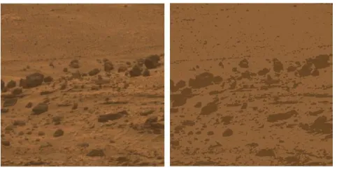
[image:4.612.212.453.150.272.2]and its color is replaced by the center value of that partition. Therefore, the image colors are quantized. For each pixel, the DCDs of a window around that pixel are calculated and presented as a feature vector corresponding to it. We assumed 8 color dominants in this research. In Fig. 1, the right image is an image in RGB domain and the left image shows the result of applying DCD.
Fig. 1. DCD of an image in RGB color space. 2.2.2. Local Color Histogram Features
Histogram is the discrete statistical probability density of the image [21]. Mars images are in RGB domain with the range 0-255 in each component. If all 256 bins are considered per R, G and B components in each histogram, it will be computationally expensive. Accordingly the range is divided to 8 equal sub-ranges for each component. To localize these features, a window is considered around each pixel and histogram of the window is computed. Therefore, each pixel of the image is mapped to a 24-dimensional feature vector in the term of local color histogram features.
2.2.3. Color Statistic Features
The first and the second moments of a window around pixels are mean and standard deviation, respectively. These features are also applied in RGB domain. The mean and standard deviation corresponding to each pixel are considered as color statistic features for each component (R, G and B). Table.1 shows the abbreviation names of all extracted features that will be used in this paper.
TABLE1
ABBREVIATION NAMES OF ALL EXTRACTED FEATURES.
Wavelet Feature Meaning Color Feature Meaning Color Feature Meaning
LH_meanL Mean of norms of L Components of LH 𝐃𝐂𝐃𝐑𝟏−𝟖 Dominant colors of R 𝑩𝒔 Std of B component
LH_meanH Mean of norms of H Components of LH 𝐃𝐂𝐃𝐆𝟏−𝟖 Dominant colors of G 𝑹𝟏−𝟖 Histogram bins of R component
LH_stdL Std of norms of L Components of LH 𝐃𝐂𝐃𝐁𝟏−𝟖 Dominant colors of B 𝑮𝟏−𝟖 Histogram bins of G component
LH_stdH Std of norms of H Components of LH 𝑹𝒎 Mean of R component 𝑩𝟏−𝟖 Histogram bins of B component
HL_meanH Mean of norms of L Components of HL 𝑮𝒎 Mean of G component
HL_meanL Mean of norms of L Components of HL 𝑩𝒎 Mean of B component
HL_stdH Std of norms of H Components of HL 𝑹𝒔 Std of R component
HL_stdL Std of norms of L Components of HL 𝑮𝒔 Std of G component
3. PIXEL CLASSIFIER BY SVM
[image:4.612.75.527.426.529.2]Fig. 2. Balancing train data for SVM classification.
4. PIXEL CLASSIFIER BY ELM
ELM originally stems from biological learning and is first proposed for the single-hidden layer feed-forward neural networks (SLFNs) and then for the generalized single-hidden layer feed-forward networks [22]. The output function of the ELM for generalized SLFNs case is computed by Eq. 2.
𝑓𝐿(𝑥) = ∑𝐿𝑖=1𝛽𝑖ℎ𝑖(𝑥) (2)
(2)
where 𝛽𝑖 is a weight between ith hidden node and the output nodes and ℎ𝑖(𝑥) is the output of the ith hidden node. It is clear that the
output functions of the hidden nodes could be different. In general, ℎ𝑖(𝑥) is a non-linear piecewise continuous function such as sigmoid, hardlimit, gaussian and multi-quadratic.
The feed-forward neural networks try to reach to smaller training errors. In ELM, both the smaller training error and the smaller norm of output weights are considered. The smaller norm of weights, the better generalization performance could be achieved. So, ELM has a higher performance in comparison with classic feed-forward networks. ELM could be expressed as an optimization problem in Eq. 3.
min: ‖𝛽‖𝑝𝜎1+ 𝐶 ‖𝐻𝛽 − 𝑇‖𝑞𝜎2 (3) (3)
where 𝜎1 and 𝜎2 are positive values and p,q=0,0.5,1,2, … . H is the matrix of h functions named as hidden layer output matrix and T is
the training data target matrix. The learning rules and mathematical theory of ELM are discussed in deeper details in [23 and 24]. ELM can be used in both classification and regression. Here, similar with SVM, ELM is used for pixel classification with a one-against-all classification scheme. For this task, ELM is trained with the training set of pixel feature vectors and then the feature vectors of unseen pixels are presented for classification. The similar idea for train data balancing, which was proposed for SVM, is applied here, too. We have used the ELM toolbox in MATLAB for ELM classification1.
5. FEATURE SELECTION
Feature selection is a discrete optimization problem which selects m features among n ones [26]. The whole search space includes all possible feature subsets of the main feature set. The number of all possible subsets is computed by Eq. (4).
∑ (𝑛 𝑠) = (
𝑛 0) + 𝑛
𝑠=0
(𝑛
1) + ⋯ + ( 𝑛 𝑛) = 2𝑛
(4)
where n represents feature vector dimension and s is the size of the current feature subset.
Alleviating the effect of the dimensionality, enhancing generalization capability, improving model interpretability and speeding up the learning process are all the benefits of removing irrelevant and redundant features from the main features [26 and 27]. Two types of feature selection methods are filter and wrapper methods. Filter methods use some metrics such as inter-class distance, probabilistic distance, class separability, entropy, error probability, consistency and correlation. In wrapper methods, classification accuracy is used for feature evaluation, show that the classifier model should be trained and tested in each step. In the filter methods, feature subset evaluation does not depend on the classification model because it does not need to train the system for each feature subset. On the other hand, wrapper methods are computationally expensive and have a risk of model over-fitting. As a result, filter methods have better generalization as well as lower complexity and over-fitting, although generally wrapper methods usually have a higher accuracy [28, 29 and 30].
5.1. Genetic Algorithm for Feature Selection
GA introduced by Holland in 1975, is a randomized heuristic search technique based on biological evolution strategies. Many complex optimization problems could be solved by GA in which chromosomes represents candidate solutions in a large population. Initial chromosomes (solutions) usually are created randomly and then next generations are generated from chromosomes with higher fitnesses. GA has been applied to our problem of interest as feature selection and feature weighting. A binary vector with the same size of the feature vector is a chromosome (solution). If the corresponding bit of a feature is one, that feature is selected and it is dropped in case it is zero. The purpose of GA in feature selection task is to find an optimal binary vector with the smallest number of 1s such that the performance of the classifier is maximized [19 and 30]. Another application of GA is feature weighting which assigns numerical weights to features instead of binary weights zero and one [31].
5.2. Ant Colony Optimization for Feature Selection
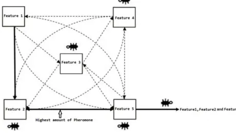
Ant colony optimization (ACO) is an iterative and probabilistic meta-heuristic method. It simulates the natural behavior of ants, consisting of mechanisms of adaptation and cooperation [32]. The ants travel among nodes of a graph and deposit pheromone for finding the shortest path. As pheromone decays over the time, each ant probabilistically prefers to follow a direction with the higher pheromone density. Accordingly the shortest path on the graph will has more pheromone and higher chance to be selected by ants and will be reinforced while pheromone of other paths’ diminished [33]. Similar to GA, ACO can be reformulated for feature selection problem by finding a path with minimum cost on a graph. In contrast with classic ACO, here, nodes in the graph represent features and the edges between nodes denote the choice of the next feature [34]. ACO starts to search for the optimal feature subset with the ant’s traverse through the graph until a minimum number of nodes are visited and traversal stop criterion is satisfied i.e. the minimum number of features with the highest classification accuracy are achieved. Any feature is allowed to be selected in each step of ant traverse, so the graph is fully connected. The pheromone update rule and transition rule of ACO algorithm can be used by a little reformulation for feature selection. In this case, pheromone and heuristic values are associated to nodes (features) rather than edges. The probability that ant k selects feature i at time step t is computed from Eq. (5).
𝑃𝑖𝑘(𝑡) = {
|𝜏𝑖(𝑡)|𝛾|𝜂𝑖|𝛿
∑𝑢∈𝐽𝑘|𝜏𝑢(𝑡)|𝛾|𝜂𝑢|𝛿 𝑖𝑓 𝑖 ∈ 𝐽 𝑘
0 𝑜𝑡ℎ𝑒𝑟𝑤𝑖𝑠𝑒
(5)
where 𝐽𝑘 is the set of features that are allowed to be added to the partial solution in case that they haven’t been visited so far. τi(t) and ηi
are the pheromone value and heuristic desirability associated with feature i respectively. γ and δ are weights of pheromone value and the heuristic information respectively[35]. The amount of deposited pheromone of ant k on feature i in step t is obtained by Eq. (6).
∆τik(t) = {ϕ. Η(S
k(t)) +ψ. (FeatutesNumber − |Sk(t)|)
FeatutesNumber if i ∈ Sk(t)
0 otherwise (6)
where FeatutesNumber is the number of all features, Sk(t) and |Sk(t)| are the feature subset and its length found by ant k at iteration 𝑡, respectively. Η(Sk(t)) is the evaluation of subset Sk(t) which is the classifier performance in this literature, 𝜙 and 𝜓 are parameters that determine the importance of the classifier performance and feature subset length, respectively. Finally, the node pheromone is updated by Eq. (7).
τi(t + 1) = (1 − ρ). τi(t) + ∑ ∆τik(t) m
k=1
+ ∆τig(t) (7)
[image:6.612.214.444.567.697.2]where m is the number of ants, 𝜌 is an evaporation rate which is constant and g is the best ant in previous iteration. It means that nodes pheromone are affected by all ants and more affected by the best ant which deposits additional pheromone on nodes. This causes the search of ants to stay around the optimal solution in the next iterations [27]. ACO feature selection is shown in Fig. 3.
5.3. The Proposed Feature Selection Methods based on ACO
Selecting the most relevant features and dropping irrelevant ones not only decreases feature vector dimension and computation cost of classifiers but also increases accuracy of such systems. In the proposed pixel classification system, feature selection is done after feature extraction stage. In feature extraction stage, a feature vector is extracted corresponding to each pixel, from a window around that pixel. In this research, two feature selection methods are proposed based on ACO.
5.3.1. The first method
It is clear that ACO feature selection is a wrapper method. In conventional ACO feature selection, each ant selects features in its path based on thier efficiency. Suppose that there are n features in feature vector. Each ant is assigned an initial feature randomly and then train the model n-1 times to select the second feature. After that, n-2 times of model training are required for the selection of the third feature.
This continues until the ant exit from its traverse. In the worst case, each ant trains the model n(n−1)2 times in each iteration. The computation cost is explosively high. Although the feature selection is done only once in the offline phase, we propose a new procedure to decrease the feature reduction cost while preserving the accuracy of classification.
At each iteration, there is a high computational cost to evaluate all ‘non-visited’ features to select one of them. Experiments show that there is no need for each ant to do that. To remedy this issue we divided features into 13 groups as shown in Table 2.
TABLE2
GROUPING FEATURES OF A PIXEL IN ACOFEATURE SELECTION.
Group Name Group Features Group Name Group Features
Group 1 LH_meanL and LH_stdL Group 8 𝑹𝒎 𝒂𝒏𝒅 𝑹𝒔
Group 2 LH_meanH and LH_stdH Group 9 𝑮𝒎 𝒂𝒏𝒅 𝑮𝒔
Group 3 HL_meanH and HL_stdH Group 10 𝑩𝒎 𝒂𝒏𝒅 𝑩𝒔
Group 4 HL_meanL nad HL_stdL Group 11 𝑹𝒊: All histogram bins of R component
Group 5 𝐃𝐂𝐃𝐑𝒊 : All color dominants of R component Group 12 𝑮𝒊: All histogram bins of G component
Group 6 𝐃𝐂𝐃𝐑𝒊 : All color dominants of G component Group 13 𝑩𝒊: All histogram bins of B component
Group 7 𝐃𝐂𝐃𝐑𝒊 : All color dominants of B component
The idea of feature grouping has this benefit that each ant only evaluates just one feature among each group. This is important since selection of each feature involves model training and testing. This idea stems from the fact that features in each group have similar effects in classification accuracy. Therefore, evaluation of all features in each group simultaneously is not necessary. On the other hand, all features of a group have a chance to be selected by ants in the next iterations. For example, if LH_meanL is a selected feature from group 1 at step k by an ant, feature LH_stdL will be a candidate to be selected by that ant from step k+1 onwards. This shows that all features have a chance to be selected by ants.
In the first proposed method, feature selection is applied to all pixel classes simultaneously. This means that the feature selection scheme tries to select the most relevant features by maximizing the classification accuracy of all pixel classes simultaneously. Therefore, the same feature subset is selected for all classes.
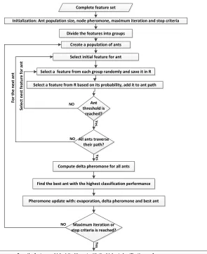
The following pseudo-code describes the proposed feature selection method in more details: 1. Initialization:
- Set the population size of ants.
- Assign each feature to a node of graph and set a random intensity of pheromone to it. - Set the maximum number of iterations.
2. Divide the features into groups.
3. Each ant builds its own solution. So, each ant should start its job from a feature(node), this feature is assigned to each ant randomly in this step and marked as ‘visited’.
4. For each ant, select one feature from each feature group randomly and save them in array 𝑎. Among features in 𝑎, select the feature with the highest probability calculated by Eq. (5) and mark this feature as ‘visited’.
5. If the ant has not reached to its proposed threshold in Eq. (8), go to 4.
Ant_Threshold = φ ∗ exp− FNN + ω ∗ expF_Measure (8)
where 𝐹𝑁 is the feature cardinality of the selected feature by the ant so far, 𝑁 is the number of all features, 𝜑 and 𝜔 are the parameters that control the effect of feature size and F_measure, respectively with restriction φ + ω = 1. Afterwards, all ants complete their search as a term of finding feature subsets.
The pheromone update is then started by three rules: 1) each ant deposits some pheromone on features. This idea stems from the natural behavior of ants. 2) Some pheromone is evaporated by time. 3) The best ant has more effect in path pheromone update since it could be a sign for other ants to follow its path in the next steps. The amount of pheromones in all features is affected by the classification accuracy and the number of features which are selected by ants.
6. For all ants, do steps 3-5.
∆pheromone(i, k) = ∝. (Model Accurarcy(k)) + β. (FeaturesNumber−FeaturesNumber(k)FeaturesNumber ) (9)
where ∆pheromone(i, k) is the amount of pheromone which is deposited by ant k on feature i, model accuracy is either Fmeasure or accuracy of the classification model (which will be explained in experimental section) trained by features founded by ant k. FeatutesNumber and FeaturesNumber(k) are the number of all features and the number of features in the path of ant k respectively. Finally, α and β are two parameters that control the relative weights of classifier performance and feature subset length, respectively, according to α + β = 1.
8. Find the best ant with the highest F-measure.
9. Pheromone update )the pheromone of all features is evaporated, all ants deposit a pheromone on the features in their paths and the best ant has extra effect on pheromone update(:
pheromonei(t + 1) = (1 − ρ). pheromonei(t) + ∑mk=1∆pheromone(i, k) + ∆pheromone(i, BestAnt)
(10)
10. Previous ants are removed and new ants are generated randomly.
11. If the stop criterion )ants follow the same path or maximum number of iteration is reached( is not achieved (go to 3, else go to 12
12. The path of ant with maximum F-measure is the best solution. 13. End
The block diagram of the first proposed feature selection algorithm is shown in Fig. 4.
5.3.2. The second method
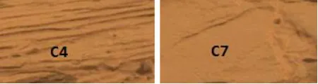
[image:8.612.195.420.432.492.2]Our first proposed feature selection method returns the most relevant features as optimal feature subset for all seven pixel classes. The first method reduces the feature vector length with maximizing Fmeasure or accuracy (to be defined later). In feature reduction phase of the first method, the main properties of all pixel classes were investigated and a feature vector including wavelet and color features was proposed. This was based on the fact that all pixels in different classes could be classified from other classes by using a single feature vector. It is clear that using an optimal feature vector for each of seven classifiers can improve the performance of the overall classification. For example, horizontal and vertical frequency components of wavelet decomposition in wavelet features are irrelevant feature for classifying pixels of class C7 while these features are strongly relevant features for classifying pixels in class C4 in Fig.5.
Fig 5. Structure of classes C4 and C7.
Accordingly in the second proposed feature selection method, an optimal feature subset is extracted for each class separately. This idea cannot be applied to ordinary classification methods such as KNNs while it can be applied to one-against-all ELMs and SVMs of all seven classes. Although this is a time consuming task, it is offline which needs to be done only once. The block diagram of this method is depicted in Fig. 6.
This type of feature selection presents an optimal feature subset for each pixel class which increases the classification accuracy in comparison with the complete feature set since all irrelevant and redundant features are omitted from the feature set in each class. The pseudo-code for the second proposed algorithm is presented as follows:
1- For each pixel class do 2-4.
2- Apply the first proposed feature selection.
Initialization: Ant population size, node pheromone, maximum iteration and stop criteria
Divide the features into groups
Select initial feature for ant
Select a feature from each group randomly and save it in R
Select a feature from R based on its probability, add it to ant path
Ant threshold is reached? Y e s NO
All ants traverse their path? NO Fo r th e n e xt a n t
Compute delta pheromone for all ants
Find the best ant with the highest classification performance
Pheromone update with: evaporation, delta pheromone and best ant Create a population of ants
Se le ct n e st f e at u re f o r an t
Complete feature set
Y
e
s
Maximum iteration or stop criteria is reached? NO
Save the features which visited by ant with the highest classification performance
Y
e
[image:9.612.174.469.68.429.2]s
Fig 4. Proposed first feature selection method based on ACO.
Complete Feature Set
A C O F ea tu re s el ec ti o n f o r cl as s 1 P ix e l C la ss ifie r w ith E LM Ants Featur e sub
set
Pheromone Update F-M
easu
re for Fe
ature s ub set P h er o m o n e Fe at u re s u bse t card in al it y Optimal Feature Subset for Class 1
…
P ix e l C la ss ifie r w ith E LM Ants Featur e subset
Pheromone Update F-M
easu
re for Fe
ature s ub set P h er o m o n e Fe at u re s ub se t ca rd in al it y A C O F ea tu re s el ec ti o n f o r cl as s 2 ...
…
P ix e l C la ss ifie r w ith E LM Ants Featur e subset
Pheromone Update F-M
easu
re for Fe
ature s ub set P h er o m o n e Fe at u
re s
u b se t ca rd in al it y A C O F ea tu re s el ec ti o n f o r cl as s 7 Optimal Feature Subset for Class 2
Optimal Feature Subset for Class 7
[image:9.612.119.461.505.672.2]6. EXPERIMENTAL SETUP
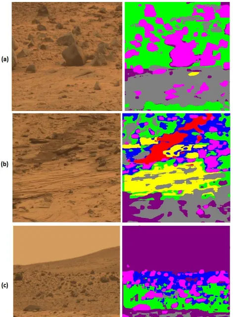
[image:10.612.220.392.153.348.2]Mars Exploration Rover Spirit dataset; which has 90 images with the size of 512x512; is used as an image dataset in this research [25]. These images are the sub images of Home Plate South panorama image. Some parts of this dataset are shown in Fig. 7. Seven classes of rocks and sands are determined in [3] for the task of pixel classification which are depicted in Table 3.
Figure.7. Some parts of Home Plate South panorama image
TABLE3 PIXEL CLASSES.
CLASS
SYMBO L
C1(ROVER TRACKS) C2(SMALL BLACK STONE AND SAND)
C3(MEDIUM BLACK STONE AND
SAND)
C4(LAYERED ROCKS)
C5(WAVE ROCKS)
C6(DARK LARGE SIZE ROCKS WITH SHADOW)
C7(FLAT ROCKS)
IMAGE
SAMPLE
To show the utility of the proposed feature selection algorithms a series of experiments are conducted. We implement the proposed algorithms on a machine with 2.26 GHz Corei7 CPU and 6GB of RAM. First, the images are zero padded by 10 pixels per side. Each pixel is windowed with a 21×21 window around it. Wavelet decomposition is computed in each window for the gray image, norm of rows and columns of LH and norm of rows and columns of HL lead to 4 vectors. The mean and standard deviation of these vectors are 8 wavelet features per pixel. In color features, the number of dominant colors is set to 8, so, 24 features are computed for R, G and B components. Also, mean and standard deviation of R, G and B components form 6 color statistic features. Finally, with 4 bins for the histogram of R, G and B, 12 features are computed. Therefore, a feature vector of dimension 50 is extracted for each pixel.
We have seven SVMs and ELMs for seven classes; each one classifies only one type of rock. To train each classifier, the pixels corresponding to each rock are considered as positive samples and the remaining pixels are considered as negative samples. Table 4 shows the number of positive and negative samples for all pixel classes used in this research. All classifiers are trained for 60% of these positive and negative pixels and the remained 40% is used as unseen data in test phase.
[image:10.612.71.551.402.505.2]TABLE4
NUMBER OF POSITIVE AND NEGATIVE SAMPLES FOR ALL PIXEL CLASSES.
Class 1 Class 2 Class 3 Class 4 Class 5 Class 6 Class 7 Number of positive samples 5651 5470 4941 10771 8682 4959 5475 Number of negative samples 5734 4365 5412 12544 9322 4566 7165
Sum 11385 9835 10353 23515 18004 9525 11640
TABLE5
PARAMETER SETTINGS FOR GA AND THE PROPOSED ALGORITHMS. Methods Iteration Population Initial
pheromone
Crossover Probability
Mutation Probability
𝛿 𝛾 𝛼 𝛽 𝜌 𝜑 𝜔
GA 100 100 - 0.6 0.008 - - - -
Proposed Algorithms
100 100 1 - - 1 1 0.6 0.4 0.3 0.1 0.9
7. EXPERIMENTAL RESULTS
Our proposed pixel classification scheme with feature selection methods are evaluated by precision, recall, Fmeasure and accuracy metrics which are computed by the Eqs. (11)-(14).
𝑃𝑟𝑒𝑐𝑖𝑠𝑖𝑜𝑛 =𝑁𝑢𝑚𝑏𝑒𝑟 𝑜𝑓 𝑎𝑙𝑙 𝑠𝑎𝑚𝑝𝑙𝑒𝑠 𝑐𝑙𝑎𝑠𝑠𝑖𝑓𝑖𝑒𝑑 𝑖𝑛𝑡𝑜 𝑝𝑜𝑠𝑖𝑡𝑖𝑣𝑒 𝑠𝑎𝑚𝑝𝑙𝑒𝑠𝑁𝑢𝑚𝑏𝑒𝑟 𝑜𝑓 𝑐𝑜𝑟𝑟𝑒𝑡𝑙𝑦 𝑐𝑙𝑎𝑠𝑠𝑖𝑓𝑖𝑒𝑑 𝑝𝑜𝑠𝑖𝑡𝑖𝑣𝑒 𝑠𝑎𝑚𝑝𝑙𝑒𝑠 (11)
𝑅𝑒𝑐𝑎𝑙𝑙 =𝑁𝑢𝑚𝑏𝑒𝑟 𝑜𝑓 𝑐𝑜𝑟𝑟𝑒𝑡𝑙𝑦 𝑐𝑙𝑎𝑠𝑠𝑖𝑓𝑖𝑒𝑑 𝑝𝑜𝑠𝑖𝑡𝑖𝑣𝑒 𝑠𝑎𝑚𝑝𝑙𝑒𝑠𝑁𝑢𝑚𝑏𝑒𝑟 𝑜𝑓 𝑝𝑜𝑠𝑖𝑡𝑖𝑣𝑒 𝑠𝑎𝑚𝑝𝑙𝑒𝑠 (12)
𝐹𝑚𝑒𝑎𝑠𝑢𝑟𝑒 = 2 × (𝑃𝑟𝑒𝑐𝑖𝑠𝑖𝑜𝑛 × 𝑅𝑒𝑐𝑎𝑙𝑙)𝑃𝑟𝑒𝑐𝑖𝑠𝑖𝑜𝑛 + 𝑅𝑒𝑐𝑎𝑙𝑙 (13)
𝐴𝑐𝑐𝑢𝑟𝑎𝑐𝑦 =𝑁𝑢𝑚𝑏𝑒𝑟 𝑜𝑓 𝑐𝑜𝑟𝑟𝑒𝑐𝑡𝑙𝑦 𝑐𝑙𝑎𝑠𝑠𝑖𝑓𝑖𝑒𝑑 𝑝𝑜𝑠𝑖𝑡𝑖𝑣𝑒 𝑎𝑛𝑑 𝑛𝑒𝑔𝑎𝑡𝑖𝑣𝑒 𝑠𝑎𝑚𝑝𝑙𝑒𝑠𝑁𝑢𝑚𝑏𝑒𝑟 𝑜𝑓 𝑎𝑙𝑙 𝑡𝑒𝑠𝑡 𝑠𝑎𝑚𝑝𝑙𝑒𝑠 (14) The results are divided into six parts. The results of classification accuracy with complete feature set, selected features by the first and second feature selection methods are reported in the following first three parts. In part 7.4, run time comparison is discussed. Statistical comparisons are reported in part 7.5 and finally segmentation results are depicted in part 7.6.
7.1. Proposed Pixel Classifier with Complete Feature Set
First experiment is done for the comparison between ELM, SVM and KNNs performances for complete feature set. Table 6 shows the precision, recall, Fmeasure and accuracy for these classifiers with complete feature set. Average results in table 6 show that ELM classifier outperforms other classifiers with complete feature set. ELM classifier with RBF kernel has the best average Fmeasure and accuracy of 0.9107 and 0.9023, respectively. It outperforms the SVM with the average Fmeasure and accuracy of 0.8726 and 0.8670, respectively and KNNs with 0.8463 and 0.8439.
TABLE6
CLASSIFICATION ACCURACY FOR COMPLETE AND OPTIMAL FEATURE SET WITH SVM,ELM AND KNNS.
Complete Feature set Selected Features by first method
Complete Feature set
Selected Features by first method
Complete Feature set
Selected Features by first method SVM MLP SVM Linear SVM Gaussian SVM MLP SVM Linear SVM Gaussian KNNs(k =5) KNNs(k =3) KNNs(k =5) KNNs (k=3) ELM RBF ELM Linear ELM RBF ELM Linear C1
Precision 0.6139 0.6553 0.6508 0.6110 0.6706 0.6453 0.6254 0.6342 0.6043 0.6234 0.6203 0.8223 0.6187 0.7786
Recall 0.9874 0.9511 0.9208 0.9867 0.9039 0.9067 0.9463 0.9533 0.9421 0.9243 0.9860 0.8906 0.9832 0.9381
Fmeasure 0.7571 0.7760 0.7626 0.7546 0.7700 0.7540 0.7530 0.7616 0.7363 0.7447 0.7615 0.8551 0.7594 0.8509 Accuracy 0.6855 0.7274 0.8536 0.6816 0.7319 0.8197 0.6920 0.7039 0.6651 0.6853 0.6935 0.8502 0.6909 0.8369
C2
Precision 0.9975 0.9991 0.9978 0.9978 0.9989 0.9876 0.9535 0.9632 0.9418 0.9612 0.9637 0.9658 0.8914 0.9611
Recall 0.8600 0.8348 0.8603 0.8526 0.8328 0.8633 0.8245 0.8043 0.8175 0.7944 0.9766 0.9427 0.9872 0.8613
Fmeasure 0.9237 0.9096 0.9240 0.9195 0.9083 0.9213 0.8843 0.8766 0.8752 0.8698 0.9701 0.9541 0.9368 0.9084 Accuracy 0.9209 0.9077 0.8750 0.9170 0.9065 0.8710 0.8800 0.8741 0.8704 0.8678 0.9665 0.9496 0.9260 0.9035
C3
Precision 0.9952 0.9981 0.9976 0.9791 0.9981 0.9765 0.9032 0.9243 0.9008 0.9150 0.9421 0.9918 0.9931 0.8518
Recall 0.7520 0.6800 0.7363 0.7770 0.6811 0.7098 0.7357 0.7466 0.7380 0.7281 0.9458 0.7942 0.7993 0.8369
Fmeasure 0.8567 0.8089 0.8473 0.8664 0.8097 0.8221 0.8108 0.8260 0.8113 0.8109 0.9439 0.8820 0.8857 0.8442 Accuracy 0.8799 0.8467 0.7922 0.8857 0.8472 0.7849 0.8362 0.8499 0.8362 0.8380 0.9464 0.8986 0.9016 0.8527
C4
Precision 0.9062 0.9436 0.8971 0.8937 0.9501 0.8876 0.8622 0.8865 0.8431 0.8734 0.9291 0.9209 0.9143 0.9642
Recall 0.9440 0.9174 0.9516 0.9541 0.9136 0.9312 0.9233 0.9543 0.8876 0.9354 0.9414 0.9180 0.9498 0.9231
C5
Precision 0.8705 0.8524 0.8965 0.8812 0.8532 0.8931 0.8565 0.8578 0.8523 0.8412 0.9178 0.8302 0.9107 0.8743
Recall 0.9357 0.9423 0.8942 0.9100 0.9301 0.8879 0.9133 0.9104 0.8831 0.9097 0.9034 0.9929 0.8991 0.9315
Fmeasure 0.9020 0.8951 0.8953 0.8954 0.8900 0.8905 0.8832 0.8833 0.8674 0.8741 0.9105 0.9043 0.9048 0.9019 Accuracy 0.9019 0.8935 0.8697 0.8974 0.8891 0.8602 0.8844 0.8840 0.8698 0.8736 0.9144 0.8986 0.9088 0.9024
C6
Precision 0.8080 0.9373 0.8024 0.7082 0.9017 0.7937 0.7976 0.9155 0.7732 0.9015 0.8985 0.8951 0.8682 0.8514
Recall 0.9020 0.5824 0.8843 0.8543 0.5647 0.8518 0.9031 0.6534 0.8942 0.6016 0.9060 0.7893 0.8725 0.7654
Fmeasure 0.8524 0.7184 0.8413 0.7744 0.6945 0.8217 0.8470 0.7625 0.8293 0.7216 0.9022 0.8388 0.8703 0.8061 Accuracy 0.8374 0.7623 0.9013 0.7409 0.7413 0.8619 0.8302 0.7882 0.8084 0.7584 0.8978 0.8421 0.8647 0.8083
C7
Precision 0.9936 0.9400 0.9989 0.9926 0.9178 0.9776 0.9878 0.9900 0.9653 0.9742 0.9448 0.9704 0.9989 0.8456
Recall 0.8087 0.8537 0.6727 0.8107 0.8494 0.6856 0.7524 0.7764 0.7442 0.7601 0.9591 0.8011 0.8454 0.9302
Fmeasure 0.8917 0.8948 0.8040 0.8925 0.8822 0.8060 0.8541 0.8702 0.8404 0.8539 0.9519 0.8776 0.9157 0.8858 Accuracy 0.9149 0.9130 0.8981 0.9154 0.9018 0.8668 0.8887 0.8998 0.8776 0.8874 0.9580 0.9033 0.9326 0.8962 Average Precision 0.8835 0.9036 0.8915 0.8662 0.8986 0.8802 0.8551 0.8816 0.8401 0.8699 0.8880 0.9137 0.8850 0.8467 Average Recall 0.8842 0.8231 0.8457 0.8779 0.8108 0.8337 0.8569 0.8283 0.8438 0.8076 0.9454 0.8755 0.8952 0.8837
Average F-measure
0.8726 0.8475 0.8568 0.8608 0.8408 0.8463 0.8463 0.8427 0.8320 0.8254 0.9107 0.8901 0.8802 0.8579
Average Accuracy
0.8670 0.8553 0.8686 0.8520 0.8508 0.8490 0.8439 0.8460 0.8284 0.8311 0.9023 0.8954 0.8800 0.8783
Optimal feature subset found by first proposed method and SVM
LH_meanL, HL_stdH, HL_stdL, DCDR1, DCDR5, DCDG4, DCDB1, Bm, Bs, R1, R6, G2,G3, B1,B4,B6,B7
Optimal feature subset found by first proposed method and KNNs
LH_stdL, HL_meanL, HL_stdL, DCDR1, DCDR7, DCDG1, DCDB1,DCDB3, Bm,Bs,R1 ,R6, G2,G3, G4,B1,B6,B8
Optimal feature subset found by first proposed method and ELM classifier
HL_stdH, HL_stdL, DCDR4, DCDR8, DCDG5, DCDB1, DCDB5, DCDB7, Bs, R4, G8, B2, B6
7.2. First Feature Selection Method
As it was mentioned before, two feature selection methods were proposed in this research. The last 3 rows of table 6 show that the first proposed method selects 13, 17 and 18 features for ELM, SVM and KNNs classifiers, respectively. From these results, it can be concluded that after dimension reduction by the first proposed method, the classification performance is preserved with a little decrease. However, we’ll show later that the main advantage of the first feature selection method is that it decreases the run time of classifiers in both train and test phases considerably. Also, there is a difference in optimal feature subsets for a system with ELM, SVM and KNNs, which stems from differences in performance of subsets in different classifiers; this leads ants to select different paths and consequently different features.
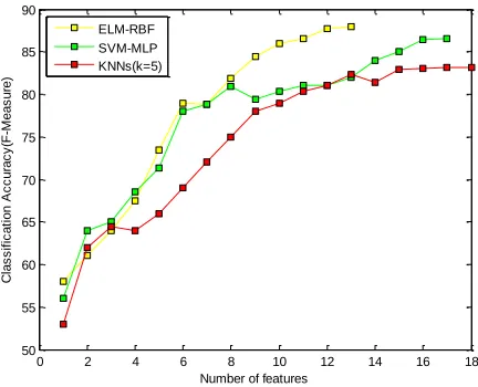
Fig. 8. Classification accuracies for highly ranked feature subsets.
7.3. Second Feature Selection Method
The second proposed feature selection method provides an optimal feature subset for each pixel classifier separately. For the majority of classifiers such as KNNs this task is not applicable, since only one model is trained for all classes and it is not possible to introduce different feature subsets for each class. In the proposed scheme, since each class has its own classifier as either ELM or SVM, it is possible to train each classifier by its own feature subset. Optimal feature subsets and reduction percents are presented in table 7. The lowest cardinality is appeared for the selected features for class C5 by ELM classifier with RBF kernel which selects 12 features among all 50 features.
[image:13.612.66.552.466.719.2]The second feature selection method decreases the dimension of the feature set and increases the classification accuracy for the majority of pixel classes. Precision, recall, Fmeasure and accuracy of the second proposed method are reported for ELM and SVM classifiers with their different kernels in Table 8. This table also shows that how performances are affected by four feature sets including complete feature set, selected features by the first and second method and selected features by genetic algorithm. The second proposed feature selection method outperforms the first proposed feature selection method and genetic algorithm-based feature selection. Furthermore, the second proposed algorithm slightly outperforms the classification performance of classifiers with complete feature set. Therefore, the second feature selection method not only decreases the feature set cardinality but also slightly increases the classification accuracy.
TABLE7
OPTIMAL FEATURE SUBSETS FOR EACH PIXEL CLASS.
ELM_RBF ELM_Linear SVM_MLP SVM_Linear
Selected Features Reduction Percent Selected Features Reduction Percent Selected Features Reduction Percent Selected Features Reduction Percent
C1 14 72% 13 74% 16 68% 17 66%
C2 13 74% 15 70% 19 62% 19 62%
C3 16 68% 17 66% 17 66% 18 64%
C4 13 74% 14 72% 19 62% 21 58%
C5 12 76% 20 60% 21 58% 20 60%
C6 14 72% 19 62% 15 70% 17 66%
C7 17 66% 16 68% 18 64% 18 64%
TABLE8
CLASSIFICATION ACCURACY FOR SECOND PROPOSED METHOD AND GA.
Complete Feature set Selected Features by first method
Selected Features by second method
Selected Features by GA
SVM_MLP ELM_RBF SVM_MLP ELM_RBF SVM_MLP ELM_RBF SVM_MLP ELM_RBF
C1
Precision 0.6139 0.6203 0.6110 0.6187 0.5889 0.6219 0.6122 0.6054
Recall 0.9874 0.9860 0.9867 0.9832 0.9892 0.9785 0.9619 0.9614
Fmeasure 0.7571 0.7615 0.7546 0.7594 0.7390 0.7604 0.7482 0.7429 Accuracy 0.6855 0.6935 0.6816 0.6909 0.6519 0.6940 0.6787 0.6698
C2
Precision 0.9975 0.9637 0.9978 0.8914 0.9960 0.9575 0.9935 0.8854
Recall 0.8600 0.9766 0.8526 0.9872 0.8883 0.9940 0.8415 0.9743
Fmeasure 0.9237 0.9701 0.9195 0.9368 0.9391 0.9754 0.9112 0.9277 Accuracy 0.9209 0.9665 0.9170 0.9260 0.9359 0.9721 0.9088 0.9156 Precision 0.9952 0.9421 0.9791 0.9931 0.9953 0.9923 0.9713 0.9834
0 2 4 6 8 10 12 14 16 18
50 55 60 65 70 75 80 85 90
Number of features
C3 Recall 0.7520 0.9458 0.7770 0.7993 0.7779 0.9443 0.7455 0.7923
Fmeasure 0.8567 0.9439 0.8664 0.8857 0.8732 0.9677 0.8436 0.8775 Accuracy 0.8799 0.9464 0.8857 0.9016 0.8922 0.9699 0.8680 0.8945
C4
Precision 0.9062 0.9291 0.8937 0.9143 0.9077 0.9396 0.8965 0.9145
Recall 0.9440 0.9414 0.9541 0.9498 0.9517 0.9714 0.9576 0.9321
Fmeasure 0.9247 0.9352 0.9229 0.9317 0.9293 0.9552 0.9260 0.9232 Accuracy 0.9290 0.9397 0.9264 0.9357 0.9330 0.9579 0.9293 0.9284
C5
Precision 0.8705 0.9178 0.8812 0.9107 0.8945 0.9587 0.8633 0.8954
Recall 0.9357 0.9034 0.9100 0.8991 0.9317 0.9111 0.9042 0.8933
Fmeasure 0.9020 0.9105 0.8954 0.9048 0.9127 0.9342 0.8833 0.8943 Accuracy 0.9019 0.9144 0.8974 0.9088 0.9141 0.9382 0.8848 0.8982
C6
Precision 0.8080 0.8985 0.7082 0.8682 0.8037 0.8854 0.7854 0.8546
Recall 0.9020 0.9060 0.8543 0.8725 0.8992 0.8986 0.8945 0.8632
Fmeasure 0.8524 0.9022 0.7744 0.8703 0.8487 0.8919 0.8364 0.8588 Accuracy 0.8374 0.8978 0.7409 0.8647 0.8332 0.8867 0.8178 0.8523
C7
Precision 0.9936 0.9448 0.9926 0.9989 0.9863 0.9912 0.9932 0.9738
Recall 0.8087 0.9591 0.8107 0.8454 0.8247 0.8965 0.7913 0.8055
Fmeasure 0.8917 0.9519 0.8925 0.9157 0.8983 0.9415 0.8808 0.8816 Accuracy 0.9149 0.9580 0.9154 0.9326 0.9191 0.9517 0.9073 0.9064 Average Precision 0.8835 0.8880 0.8662 0.8850 0.8817 0.9066 0.8736 0.8732 Average Recall 0.8842 0.9454 0.8779 0.8952 0.8946 0.9406 0.8709 0.8888 Average F-measure 0.8726 0.9107 0.8608 0.8802 0.8771 0.9172 0.8613 0.8722 Average Accuracy 0.8670 0.9023 0.8520 0.8800 0.8684 0.9100 0.8563 0.8664
7.4. Run Time Comparison
Run time is so important especially for the on-board applications of Mars image segmentation. Here, the run time is considered for both train and test phases. Table 9 reports the run time of train and test phases in three classifiers with complete feature set for different parameters. Although KNN has no training time, its classification accuracy is very lower than SVM and ELM. Generally, ELM with linear kernel has the lowest run time with an average of 4402ms and 180ms for train and test phases respectively.
The first proposed feature selection algorithm selects the most relevant features for all classes simultaneously. Train and test samples of all classes are involved in steps 4, 5 and 7 of this algorithm while in the second feature selection algorithm the train and test samples of only one class are involved at the same time. The run times of the first and second feature selection algorithms are 1286 and 353 seconds, respectively. Note that 353 seconds is only for one class in the second feature selection method. Feature selection for other classes can be run with parallel procedures. These run times are the average run times of using different classifiers in feature selection process. It should be noted that the proposed feature selection algorithms are done once in offline phase and then selected features will be used for the train and test phases of classifiers. Therefore, their run times are not the concern for pixel classification application. The main advantage of the proposed feature selection methods is dimension reduction which decreases the run time considerably. Therefore, we also have reported the run time of classifiers with selected features by two proposed feature selection algorithms in train and test phases in Fig. 9 and Fig. 10, respectively. For these two figures some abbreviations are used for each bar. For example, ‘SVM-Linear-Comp’ means that SVM classifier with linear kernel is used for complete feature set and ‘SVM-Linear-First’ means that SVM classifier with linear kernel is used for selected features by the first proposed method. For train run times, only ELM and SVM are compared since KNNs has no train run time. It is concluded from these figures that classifiers with selected features by feature selection methods have lower run times in train and test phases. Another conclusion is that each classifier with selected features from the first and second feature selection methods has the same run time. However, the main advantage of the second proposed method is its higher accuracy which was reported in Table 8 in more details.
TABLE9
RUN TIME OF SVM,KNN AND ELM FOR COMPLETE FEATURE SET.
ELM_RBF ELM_Linear SVM_MLP SVM_Linear KNNs(k=3) KNNs(k=5) C1 Train time(ms2) 2734 2032 7554 20041 - -
Test time(ms) 719 106 368 125 5228 7242 C2 Train time(ms) 1677 1172 2471 1233 - -
Test time(ms) 463 72 133 46 4338 4845
C3 Train time(ms) 2244 1562 6792 11011 - - Test time(ms) 610 89 316 106 6876 7929 C4 Train time(ms) 18318 12954 25054 32767 - -
Test time(ms) 4150 442 1214 432 26545 29415
C5 Train time(ms) 11588 9046 17350 29637 - - Test time(ms) 2333 320 811 352 18337 20980 C6 Train time(ms) 1882 1254 5594 6517 - -
Test time(ms) 519 88 291 98 5842 6835
C7 Train time(ms) 4608 2795 9603 23052 - - Test time(ms) 1204 147 509 166 11589 14516
Average Train Time 6150 4402 10631 17751 - - Average Test Time 1428 180 520 189 11250 13108
Fig. 9. Train run time for ELM and SVM classifiers with selected features of first and second feature selection methods.
Fig. 10. Test run time for ELM, SVM and KNNs classifiers with selected features of first and second feature selection methods.
7.5. Statistical Comparison
comparison too. In this research, for overall comparison of methods, two sets with seven elements should be compared. Therefore, parametric statistical tests aren’t applicable here and pairwise U-Mann-Whitney test is used which is a non-parametric test. In this test, the null hypothesis is that two samples come from the same population against an alternative hypothesis with the meaning that the two samples are from different populations. This test provides the confidence level for the differences between sets as well as a mean rank for each set. We first determine that two sets are different with a confidence level and then determine the better set which is the set with higher mean rank. Different pairwise comparisons between classifiers with different feature sets are reported in table 10. This table shows the mean rank and confidence level between each two sets and its last column determines which set is statistically better than another. The confidence level threshold of 90% is considered. The main conclusion is that ELM with the complete feature set outperforms other classifiers statistically with a confidence level of 94%. Furthermore, the classification performance of classifiers with complete feature set and with selected features are statistically the same. This means that after dimension reduction the classification performance isn’t decreased statistically. Although the mean rank of classifier performances with the selected features by second feature selection method is higher than classifier performances with complete feature set, its confidence level is very low and under predefined threshold. Therefore, we reported that none of which is better than other. Finally, it is resulted that the second proposed feature selection method outperforms the genetic algorithm with the confidence level of 95.2%.
TABLE10
PAIRWISE STATISTICAL COMPARISON OF ALL METHODS.
Comparative Mean Ranks
Confidence Level Which one is better
statistically?
F-Measure
Complete Feature Set
ELM and SVM 9.57 and 5.43 94.4% ELM
ELM and KNNs 10.14 and 4.84 98.2% ELM
First Method and Complete
ELM_Com and ELM_First 9.00 and 6.00 82% None
SVM_Com and SVM_First 7.86 and 7.14 25.1% None
KNNs_Com and KNNs_First 8.43 and 6.57 59.4% None
Second Method and Complete
ElM_Com and ELM_Second 7.14 and 7.86 25.1% None
SVM_Com and SVM_Second 7.14 and 7.86 25.1% None
Second Method and GA
ELM_Second and ELM_GA 9.71 and 5.29 95.2% ELM_Second
SVM_Second and SVM_GA 8.43 and 6.57 59.4% None
Accuracy
Complete Feature Set
ELM and SVM 9.14 and 5.86 85.8 None
ELM and KNNs 10.14 and 4.86 98.2 ELM
First Method and Complete
ELM_Com and ELM_First 9 and 6 82% None
SVM_Com and SVM_First 7.71 and 7.29 15.2% None
KNNs_Com and KNNs_First 8.79 and 6.21 75% None
Second Method and Complete
ElM_Com and ELM_Second 6.86 and 8.14 43.5% None
SVM_Com and SVM_Second 7.14 and 7.76 25.1% None
Second Method and GA
ELM_Second and ELM_GA 9.43 and 5.57 91.5% ELM_Second
SVM_Second and SVM_GA 8.57 and 6.43 66.2% None
7.6. Segmentation Results
8. CONCLUSION
Home plate south panorama images contain information about Mars, taken by Mars rover, a robot which explores on Mars surface. In this paper, a new pixel classification scheme was proposed which leads to Mars image segmentation. Firstly, each pixel is windowed and mapped to a feature vector including wavelet and color features. The type of extracted features was proposed by the way that all pixel classes could be discriminated from other classes and appropriate segmentation of images are achieved. Then, most relevant features among complete feature set were selected by two proposed feature selection schema based on ACO. Finally, optimal feature sets were presented for the classifiers for pixel classification. Classification of pixels segments the images into pixel groups. Our proposed model for image segmentation was compared with other methods; results showed that the proposed pixel classification scheme with complete feature set and ELM classifier outperforms other classifiers include SVM and KNNs in both accuracy and run time. Furthermore, the first feature selection method presents a feature subset which decreases the run times and preserves the accuracies of not only ELM classifier but also SVM and KNNs classifiers. Finally, the second proposed feature selection method selects an optimal feature subset for each pixel class separately. This method decreases the run time and increases the accuracies of most of classifiers simultaneously. It also outperforms the first proposed feature selection method and genetic algorithm-based feature selection. For future works, the performance of the proposed approaches can be evaluated by taking into account other classifiers such as artificial neural networks and decision trees. Other feature selection methods can be improved and applied to such systems. In addition, intrinsic property of data such as Relief weights can be used in population-based techniques such as ACO, GA and Particle swarm optimization (PSO) algorithms to increase convergence speed. Finally, other features like shape and texture features and color features in other color systems can also be applied for pixel classification task.
REFERENCES
[1] Xue, Yansong, Shuanggen Jin, and Yi Yang. "Mineral components at Martian Gale region from Mars Reconnaissance Orbiter CRISM images."
[2] Castano, R., Judd, M., Estlin, T., Anderson, R. C., Gaines, D., Castaño, A., ... & Wagstaff, K. (2005). Current results from a rover science data analysis system. In Aerospace Conference, 2005 IEEE (pp. 356-365). IEEE.
[3] Shang, C., & Barnes, D. (2013). Fuzzy-rough feature selection aided support vector machines for mars image classification. Computer Vision and Image Understanding, 117(3), 202-213.
[4] Pang, Y., Zhu, H., Li, X., & Pan, J. (2016). Motion Blur Detection with an Indicator Function for Surveillance Machines, vol. 63, no. 9, pp. 5592-5601.
[5] Pang, Y., Zhu, H., Li, X., & Li, X. (2016). Classifying discriminative features for blur detection, vol. 46, no. 10, pp. 2220-2227.
[6] De Cooman, G. (2005). A behavioural model for vague probability assessments. Fuzzy sets and systems, 154(3), 305-358. [7] Huang, K., & Aviyente, S. (2008). Wavelet feature selection for image classification. Image Processing, IEEE Transactions
on, 17(9), 1709-1720.
[8] Kachanubal, T., & Udomhunsakul, S. (2008). Rock textures classification based on textural and spectral features. Int J Comput Intell, 4, 240-246.
[9] Puig, D., & Garcia, M. A. (2006). Automatic texture feature selection for image pixel classification. Pattern Recognition, 39(11), 1996-2009.
[10]Kashef, S., & Nezamabadi-pour, H. (2015). An advanced ACO algorithm for feature subset selection. Neurocomputing, 147, 271-279.
[11]Yong, Z., Dun-wei, G., & Wan-qiu, Z. (2015). Feature selection of unreliable data using an improved multi-objective PSO algorithm. Neurocomputing.
[12] Alexandre, E., Cuadra, L., Salcedo-Sanz, S., Pastor-Sánchez, A., & Casanova-Mateo, C. (2015). Hybridizing Extreme Learning Machines and Genetic Algorithms to select acoustic features in vehicle classification applications. Neurocomputing, 152, 58-68.
[13]Diao, R., & Shen, Q. (2012). Feature selection with harmony search. Systems, Man, and Cybernetics, Part B: Cybernetics, IEEE Transactions on, 42(6), 1509-1523.
[14]d Gundimada, S., Asari, V. K., & Gudur, N. (2010). Face recognition in multi-sensor images based on a novel modular feature selection technique. Information Fusion, 11, 124-132
[15]Jensen, R. (2005). Combining rough and fuzzy sets for feature selection. Ph.D. thesis, University of Edinburgh.
[16]Rashno, A., SadeghianNejad, H., & Heshmati, A. (2013). Highly Efficient Dimension Reduction for Text-Independent Speaker Verification Based on Relieff Algorithm and Support Vector Machines”. International Journal of Signal Processing, Image Processing and Pattern Recognition, 6(1).
[18] Shang, C., & Barnes, D. (2010, September). Combining support vector machines and information gain ranking for classification of mars mcmurdo panorama images. In Image Processing (ICIP), 2010 17th IEEE International Conference on (pp. 1061-1064). IEEE.
[19]Dunn, P. F. (2014). Measurement and data analysis for engineering and science. CRC press.
[20]ISO/IEC 15938-3/FDIS Information Technology—Multimedia Content Description Interface—Part 3 Visual Jul. 2001, ISO/IEC/JTC1/SC29/WG11 Doc. N4358.
[21]Gonzalez, R., Woods R.E. (2008). Digital Image Processing and Scene Analysis, third edition, Prentice Hall,.
[22]Huang, Guang-Bin. "An insight into extreme learning machines: random neurons, random features and kernels." Cognitive Computation 6.3 (2014): 376-390.
[23]Cao, Jiuwen, and Zhiping Lin. "Extreme Learning Machines on High Dimensional and Large Data Applications: A Survey." Mathematical Problems in Engineering 501 (2015): 103796.
[24]Huang, Gao, et al. "Semi-supervised and unsupervised extreme learning machines." Cybernetics, IEEE Transactions on 44.12 (2014): 2405-2417.
[25]http://marswatch.astro.cornell.edu/pancam_instrument/home_plate_south.html.
[26]Mladenić, D. (2006). Feature selection for dimensionality reduction (pp. 84-102). Springer Berlin Heidelberg.
[27] Nemati, S., & Basiri, M. E. (2011). Text-independent speaker verification using ant colony optimization-based selected features. Expert Systems with Applications, 38(1), 620-630.
[28] Peng, Hanchuan, Fulmi Long, and Chris Ding. "Feature selection based on mutual information criteria of max-dependency, max-relevance, and min-redundancy." Pattern Analysis and Machine Intelligence, IEEE Transactions on 27.8 (2005): 1226-1238.
[29]17 Liu, H., & Motoda, H. (Eds.). (2007). Computational methods of feature selection. CRC Press.
[30]Yang, J., & Honavar, V. (1998). Feature subset selection using a genetic algorithm. In Feature extraction, construction and selection (pp. 117-136). Springer US.
[31]Beddoe, G. R., & Petrovic, S. (2006). Selecting and weighting features using a genetic algorithm in a case-based reasoning approach to personnel rostering. European Journal of Operational Research, 175(2), 649-671.
[32]Dorigo, M., Birattari, M., & Stutzle, T. (2006). Ant colony optimization. Computational Intelligence Magazine, IEEE, 1(4), 28-39.
[33]Al-Ani, A. (2005, February). Ant Colony Optimization for Feature Subset Selection. In WEC (2) (pp. 35-38).
[34]Huang, C. L. (2009). ACO-based hybrid classification system with feature subset selection and model parameters optimization. Neurocomputing, 73(1), 438-448.