ELLIPTICAL COST-SENSITIVE DECISION TREE
ALGORITHM - ECSDT
MOHAMMAD ELBADAWI KASSIM
SCHOOL OF COMPUTING, SCIENCE AND ENGINEERING
INFORMATICS RESEARCH CENTRE, UNIVERSITY OF
SALFORD, MANCHESTER, UK
i
TABLE OF CONTENTS ... i
LIST OF FIGURES ... iii
LIST OF TABLES ... v
LIST OF ABBREVIATIONS ... viii
ACKNOWLEDGEMENTS ... x
ABSTRACT ... xi
Chapter 1 : INTRODUCTION ... 1
1.1 Background ... 1
1.2 Motivation ... 3
1.3 Problem Definition ... 4
1.4 Aims and Objectives ... 4
1.5 Research Methodology ... 5
1.5.1 Quantitative Research Methodology ... 6
1.6 Research Contributions ... 8
1.7 Outline of Thesis ... 8
Chapter 2 : GENERAL BACKGROUNDS ... 10
2.1 Background of Supervised Learning ... 10
2.1.1 Basic Concepts of Supervised Learning ... 12
2.1.2 Developing Supervised Learning Algorithms ... 13
2.1.3 Cross-Validation ... 15
2.2 Background of Decision Tree Learning ... 17
2.2.1 Feature Selection Methods for Decision Trees ... 19
2.2.2 DTs Performance Measures... 21
2.3 Confusion and Cost Matrices ... 24
Chapter 3 : THE LITERATURE REVIEW ... 28
3.1 Cost-Sensitive Learning ... 28
3.1.1 Cost-Sensitive Learning Theories and Strategies ... 29
ii
3.4 Evolutionary Optimization Methods ... 45
3.5 Summary of the Literature Review ... 54
Chapter 4 : DEVELOPMENT OF THE NEW ALGORITHM ... 56
4.1 Introduction ... 56
4.2 Formulation of Cost-Sensitive Learning as an Optimization Problem ... 57
4.3 Constructing Trees from Ellipses ... 62
4.4 Implementing ECSDT in the MOEA Framework ... 68
4.5 Illustrative Examples of How (ECSDT) Works: ... 72
Chapter 5 : EMPIRICAL EVALUATION OF THE NEW ALGORITHM ... 76
5.1 Datasets ... 76
5.2 Comparative Algorithms ... 78
5.3 Empirical Evaluation ... 80
5.3.1 Empirical Comparison Based on Accuracy ... 82
5.3.2 Empirical Comparison Based on Cost ... 93
5.3.3 Empirical Comparison Based on Both Accuracy and Cost ... 111
Chapter 6 : CONCLUSION AND FUTURE WORK ... 128
6.1 Evaluating the Achievement of the Objectives ... 129
6.2 Future Work ... 131
REFERENCES ... 134
APPENDIX – A: Details of the Datasets Used in the Research ... 142
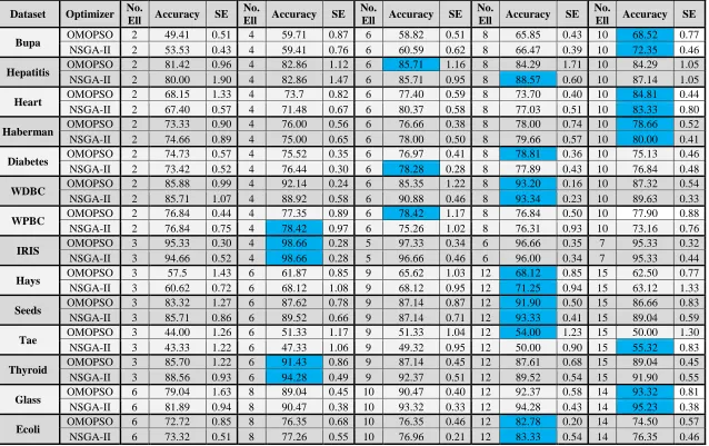
APPENDIX – B: Results of the Empirical Comparison Based on Accuracy ... 149
APPENDIX – C: Results of the Empirical Comparison Based on Cost ... 153
iii
Figure 1.1: Nonlinear classification (example - 1) ... 3
Figure 1.2: Nonlinear classification (example - 2) ... 3
Figure 1.3: Linear classification for (example - 1) ... 3
Figure 1.4: Linear classification for (example - 2) ... 3
Figure 1.5: Elliptical classification for (example - 1) ... 4
Figure 1.6: Elliptical classification for (example - 2) ... 4
Figure 1.7: Methodology stages ... 7
Figure 3.1: Classification problem before applying Kernel tricks ... 41
Figure 3.2: Classification problem after applying Kernel tricks ... 41
Figure 3.3: The flowchart of NSGA-II general procedure ... 49
Figure 3.4: The pseudo code of general single-objective PSO... 51
Figure 3.5: The pseudo code of general multi-objective PSO ... 53
Figure 4.1: Linear classification ... 57
Figure 4.2: Elliptical classification ... 57
Figure 4.3: One level placement of ellipses ... 60
Figure 4.4: Multi-levels placement of ellipses ... 60
Figure 4.5: The outline for the (ECSDT) algorithm ... 61
Figure 4.6: The outline for constructing the DT using (ECSDT) ... 64
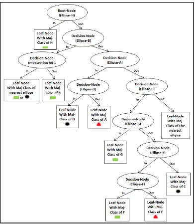
Figure 4.7: The decision tree for the example shown in Fig (4.4) ... 65
Figure 4.8: The outline for classifying new examples using ECSDT ... 66
Figure 4.9: Examples of classifying new instances using ECSDT... 67
Figure 4.10: The pseudo code of the top-level for the new algorithm ... 70
Figure 4.11: The pseudo code of the optimisation process ... 71
Figure 4.12: Hypothetical multiclass classification problem ... 72
Figure 4.13: Elliptical classification example-1 ... 72
Figure 4.14: Assigning examples to ellipses ... 73
Figure 4.15: Elliptical classification example-2 ... 74
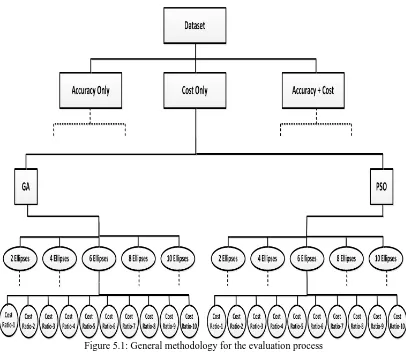
Figure 5.1: General methodology for the evaluation process ... 82
Figure 5.2: Accuracy comparison (Accuracy-based aspect) ... 87
Figure 5.3: DT-size comparison (Accuracy-based aspect) ... 87
Figure 5.4: Line chart for the Accuracy-based results (Bupa) ... 89
iv
Figure 5.8: Cost comparison (Cost-based aspect) ... 99
Figure 5.9: Accuracy comparison (Cost-based aspect) ... 100
Figure 5.10: DT-size comparison (Cost-based aspect) ... 100
Figure 5.11: Bupa cost comparison for the Cost-Based aspect ... 103
Figure 5.12: Bupa accuracy comparison for the Cost-Based aspect ... 103
Figure 5.13: Bupa DT-size comparison for the Cost-Based aspect ... 104
Figure 5.14: IRIS cost comparison for the Cost-Based aspect ... 107
Figure 5.15: IRIS accuracy comparison for the Cost-Based aspect ... 107
Figure 5.16: IRIS DT-size comparison for the Cost-Based aspect... 108
Figure 5.17: Ecoli cost comparison for the Cost-Based aspect ... 110
Figure 5.18: Ecoli accuracy comparison for the Cost-Based aspect ... 110
Figure 5.19: Ecoli DT-size comparison for the Cost-Based aspect ... 111
Figure 5.20: Cost comparison (Accuracy + Cost) based aspect ... 116
Figure 5.21: Cost comparison (Accuracy + Cost) based aspect ... 116
Figure 5.22: Accuracy comparison (Accuracy + Cost) based aspect ... 117
Figure 5.23: DT-size comparison (Accuracy + Cost) based aspect ... 117
Figure 5.24: Bupa cost comparison for the (Accuracy + Cost) based aspect ... 120
Figure 5.25: Bupa accuracy comparison for the (Accuracy + Cost) based aspect ... 120
Figure 5.26: Bupa DT-size comparison for the (Accuracy + Cost) based aspect ... 121
Figure 5.27: IRIS cost comparison for the (Accuracy + Cost) based aspect ... 124
Figure 5.28: IRIS accuracy comparison for the (Accuracy + Cost) based aspect ... 124
Figure 5.29: IRIS DT-size comparison for the (Accuracy + Cost) based aspect ... 124
Figure 5.30: Ecoli cost comparison for the (Accuracy + Cost) based aspect ... 127
Figure 5.31: Ecoli accuracy comparison for the (Accuracy + Cost) based aspect ... 127
v
Table 2.1: The confusing matrix for binary classification problem ... 25
Table 2.2: The cost matrix for binary classification problem... 25
Table 2.3: The confusion matrix for a 3-classes classification problem ... 25
Table 2.4: The cost matrix for a 3-classes classification problem... 25
Table 2.5: Confusion matrix (Example-1) ... 26
Table 2.6: Cost matrix (Example-1) ... 26
Table 2.7: Confusion matrix (Example-2) ... 27
Table 4.1: The confusion matrix obtained when applying ECSDT for example-1 ... 74
Table 4.2: The confusion matrix obtained for example-2 ... 74
Table 4.3: The cost matrix of (example-1 and example-2) ... 75
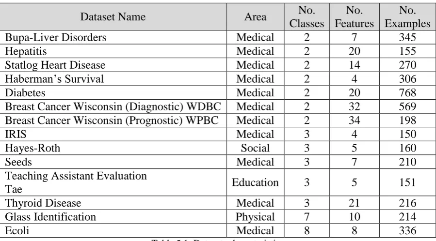
Table 5.1: Datasets characteristics... 77
Table 5.2: Accuracy-based results for all datasets using different number of ellipses when ECSDT is applied ... 85
Table 5.3: Accuracy-based Results for all datasets when applying different algorithms.... 86
Table 5.4: Accuracy-based results (Bupa) ... 88
Table 5.5: Accuracy-based results (IRIS)... 90
Table 5.6: Accuracy-based results (Ecoli) ... 92
Table 5.7: Misclassification cost ratios used in all experiments ... 94
Table 5.8: Cost-based results for all datasets using different number of ellipses ... 97
Table 5.9: Cost-based results for all datasets when applying different algorithms ... 98
Table 5.10: Bupa Cost-Based results for each number of ellipses (ECSDT+OMOPSO) . 101 Table 5.11: Bupa Cost-Based results for each number of ellipses (ECSDT+NSGA-II) ... 101
Table 5.12: Bupa Cost-Based results obtained by the comparative algorithms ... 102
Table 5.13: IRIS Cost-Based results for each number of ellipses (ECSDT+OMOPSO) .. 105
Table 5.14: IRIS Cost-Based results for each number of ellipses (ECSDT+NSGA-II) ... 105
Table 5.15: IRIS Cost-Based results obtained by the comparative algorithms (IRIS) ... 106
Table 5.16: Ecoli Cost-Based results for each number of ellipses (ECSDT+OMOPSO) . 108 Table 5.17: Ecoli Cost-Based results for each number of ellipses (ECSDT+NSGA-II) ... 109
Table 5.18: Ecoli Cost-Based results obtained by the comparative algorithms ... 109
vi Table 5.21: Bupa (Accuracy + Cost) based results for each number of ellipses
(ECSDT+OMOPSO) ... 118
Table 5.22: Bupa (Accuracy + Cost) based results for each number of ellipses (ECSDT+NSGA-II) ... 118
Table 5.23: Bupa (Accuracy + Cost) based results obtained by the comparative algorithms ... 119
Table 5.24: IRIS (Accuracy + Cost) based results for each number of ellipses (ECSDT+OMOPSO) ... 122
Table 5.25: IRIS (Accuracy + Cost) based results for each number of ellipses (ECSDT+NSGA-II) ... 122
Table 5.26: IRIS (Accuracy + Cost) based results obtained by the comparative algorithms ... 123
Table 5.27: Ecoli (Accuracy + Cost) based results for each number of ellipses (ECSDT+OMOPSO) ... 125
Table 5.28: Ecoli (Accuracy + Cost) based results for each number of ellipses (ECSDT+NSGA-II) ... 125
Table 5.29: Ecoli (Accuracy + Cost) based results obtained by the comparative algorithms ... 126
Table Apx-B-1: Bupa Accuracy-based results ... 149
Table Apx-B-2: Hepatitis Accuracy-based results ... 149
Table Apx-B-3: Heart Accuracy-based results ... 149
Table Apx-B-4: Haberman Accuracy-based results ... 149
Table Apx-B-5: Diabetes Accuracy-based results... 150
Table Apx-B-6: WDBC Accuracy-based results... 150
Table Apx-B-7: WPBC Accuracy-based results ... 150
Table Apx-B-8: IRIS Accuracy-based results ... 150
Table Apx-B-9: Hayes Accuracy-based results... 151
Table Apx-B-10: Seeds Accuracy-based results ... 151
Table Apx-B-11: Tae Accuracy-based results... 151
Table Apx-B-12: Thyroid Accuracy-based results ... 151
Table Apx-B-13: Glass Accuracy-based results ... 152
vii
Table Apx-C-3: Heart Cost-based results ... 155
Table Apx-C-4: Haberman Cost-based results ... 156
Table Apx-C-5: Diabetes Cost-based results ... 157
Table Apx-C-6: WDBC Cost-based results ... 158
Table Apx-C-7: WPBC Cost-based results ... 159
Table Apx-C-8: IRIS Cost-based results ... 160
Table Apx-C-9: Hays Cost-based results ... 161
Table Apx-C-10: Seeds Cost-based results ... 162
Table Apx-C-11: Tae Cost-based results ... 163
Table Apx-C-12: Thyroid Cost-based results ... 164
Table Apx-C-13: Glass Cost-based results ... 165
Table Apx-C-14: Ecoli Cost-based results ... 166
Table Apx-D-1: Bupa Accuracy + Cost based results ... 167
Table Apx-D-2: Hepatitis Accuracy + Cost based results ... 168
Table Apx-D-3: Heart Accuracy + Cost based results ... 169
Table Apx-D-4: Haberman Accuracy + Cost based results ... 170
Table Apx-D-5: Diabetes Accuracy + Cost based results ... 171
Table Apx-D-6: WDBC Accuracy + Cost based results ... 172
Table Apx-D-7: WPBC Accuracy + Cost based results ... 173
Table Apx-D-8: IRIS Accuracy + Cost based results ... 174
Table Apx-D-9: Hays Accuracy + Cost based results ... 175
Table Apx-D-10: Seeds Accuracy + Cost based results ... 176
Table Apx-D-11: Tae Accuracy + Cost based results ... 177
Table Apx-D-12: Thyroid Accuracy + Cost based results ... 178
Table Apx-D-13: Glass Accuracy + Cost based results ... 179
viii
Acc Accuracy
AdaBoost AdaBoost (Adaptive Boosting)
ADTree Alternating Decision Tree
BFTree Best-First Tree
BPNN Back Propagation Neural Network
C.S.C+J48 CostSensitiveClassifier with J48
C.S.C+NBTree CostSensitiveClassifier with Naive Bayesian Tree
CART Classification And Regression Trees
CSC CostSensitive Classifier
CSDTWMCS Cost-Sensitive Decision Trees with Multiple Cost Scales
CS-ID3 Cost-Sensitive Iternative Dichotomizer 3
CSNB Cost-Sensitive Naive Bayes
CSNL Cost-sensitive Non-linear Decision Tree
CSTree Cost-Sensitive Tree
CV Cross-Validation
DAGSVM Directed Acyclic Graph Support Vector Machine
DB2 Divide-by-2
DDAG Decision Directed Acyclic Graph
DT Decision Tree
EAs Evolutionary algorithms
ECCO Evolutionary Classifier with Cost Optimization
ECM Expected Cost of Misclassification
ECOC Error Correcting Output Coding
ECSDT Elliptical Cost Sensitive Decision Tree
ECSDT +GA Elliptical Cost-Sensitive Decision Tree with Genetic Algorithm
ECSDT +PSO Elliptical Cost-Sensitive Decision Tree with Partial Swarm Optimization
Eq Equation
FDA Fisher Discriminant Analysis
FN False Negative
FP False Positive
GA Genetic Algorithm
GBSE Gradient Boosting with Stochastic Ensembles
GDT-MC Genetic Decision Tree with Misclassification Costs
GP Genetic Programming
HKWDA Heteroscedastic Kernel Weighted Discriminant Analysis
ICET Inexpensive Classification with Expensive Tests
ICF Information Cost Function
ID3 Iternative Dichotomizer 3
IG Information Gain
LADTree Logical Analysis of Data Tree
ix
ML Machine Learning
MLSVM Mixture of Linear Support Vector Machines
MNCS_DT Non-linear Cost-sensitive Decision Tree for Multiclassification
MOEA Multi-Objective Evolutionary Algorithms
MOOP Multi-Objective Optimization Problem
NB Naive Bayesian
NBT Naive Bayesian Tree
NSGA-II Nondominated Sorting Genetic Algorithm II
OMOPSO Optimum Multi-Objective Particle Swarm Optimization
PPV Positive Predictive Value
PSO Particle Swarm Optimization
PSOC4.5 Particle Swarm Optimization with C4.5 algorithm
PSO-SVM Particle Swarm Optimization with Support Vector Machines
RepTree Reduced Error Pruning Tree
SOM Self-Organizing Map
SRM Structural Risk Minimization
SVM Support Vector Machine
SVM-BDT Support Vector Machines utilizing Binary Decision Tree
TCSDT Test Cost-sensitive Decision Tree
TN True Negative
TP True Positive
UCI University of California, Irvine
x First of all, I would like to express my deep thanks and gratitude to Allah Almighty for his help and support in completing this research journey.
I would like also to take this opportunity to express my deep thanks and gratitude to my supervisor Prof. Sunil Vadera who was always ready to help and provide me with a continuous support and guidance throughout the entire period of this research.
Very special thanks to all my family for their continuous love and support, most especially, My father, for his continuous prays for me.
xi Cost-sensitive multiclass classification problems, in which the task of assessing the impact of the costs associated with different misclassification errors, continues to be one of the major challenging areas for data mining and machine learning.
The literature reviews in this area show that most of the cost-sensitive algorithms that have been developed during the last decade were developed to solve binary classification problems where an example from the dataset will be classified into only one of two available classes.
Much of the research on cost-sensitive learning has focused on inducing decision trees, which are one of the most common and widely used classification methods, due to the simplicity of constructing them, their transparency and comprehensibility.
A review of the literature shows that inducing nonlinear multiclass cost-sensitive decision trees is still in its early stages and further research could result in improvements over the current state of the art. Hence, this research aims to address the following question:
How can non-linear regions be identified for multiclass problems and utilized to construct decision trees so as to maximize the accuracy of classification, and minimize misclassification costs?
This research addresses this problem by developing a new algorithm called the Elliptical Cost-Sensitive Decision Tree algorithm (ECSDT) that induces cost-sensitive non-linear (elliptical) decision trees for multiclass classification problems using evolutionary optimization methods such as particle swarm optimization (PSO) and Genetic Algorithms (GAs). In this research, ellipses are used as non-linear separators, because of their simplicity and flexibility in drawing non-linear boundaries by modifying and adjusting their size, location and rotation towards achieving optimal results.
1
Chapter 1
: INTRODUCTION
1.1 Background
Nowadays, due to the vast amounts of information available and the rapid development in the use of computers and modern information technologies, the optimal use of these data is a challenge for decision-makers who are struggling when they have to make the right decisions to ensure the best results whilst simultaneously achieving low costs associated with those decisions. Machine Learning is one of the most prominent fields of science that has been employed to assist decision-makers, scientists and researchers in various branches of science and knowledge discovery. Machine learning is the field through which decision-making criteria are learned and developed using the available data and utilizing information and knowledge that has been acquired from previous experiences in the field of study. It has become one of the most widely used subfields of computer science, largely because it is used in a wide variety of applications. Some examples of applications that use machine learning include processing natural language, speech and sound recognition, fraud detection, documents checking, computer visibility, and medical diagnosis. With the expansion of the use of the internet and social networking media, the amount of data exchanged between users has increased significantly. Because of these factors, there has been significant progress in the field of machine learning which provides many tools that can intelligently gather and analyse different types of data and then utilise this experience to produce valuable information.
2 objective of most of these techniques was only to minimize the error rate and ignored costs associated with any type of misclassification as they assume that the costs of all types of misclassification are equal.
Cost-sensitive learning is one of the most challenging recent research topics in data mining
and machine learning that strives to develop solutions that help decision-makers make the right decisions at the lowest possible costs. For example, in real-world medical diagnostics,
classifying a person with a serious illness as a healthy person is more critical and more costly
than classifying a healthy person as a sickly one where the error in the first case may cost the
life of the patient, while in the second case the cost will be limited to the cost that is associated
to some extra medical tests.
During the last decades, many cost-sensitive learning methods and algorithms have been developed in this field. Lomax and Vadera (2011) present a comprehensive survey of existing studies and algorithms that have been introduced for the purpose of cost-sensitive decision tree learning. Their review identified over 50 algorithms for cost-sensitive learning, most of which focus on binary classification problems. Most authors tackle multiclass problems by converting them into many binary-class sub-problems and then applying the normal binary classifiers on them (Aly 2005) but intuitively the disadvantage of such methods is that they can give fairly unreliable results as if only one of the binary classifiers make a mistake, then it is possible that the entire prediction is wrong.
Vadera (2010) notes that the majority of recent cost-sensitive decision tree induction algorithms, such as in WEKA and R, attempt to deal with classification problems by utilizing linear separators, such as using straight lines, or what is known as axis parallel splits to separate out non-linear regions. Clear visualisation is another challenge facing the current cost-sensitive algorithms. It has been stated in (Ankerst et al. 1999), that the effective visualization of large decision trees particularly in the learning process still requires efficient tools that make the visualization more clear and easy to understand.
3 1.2 Motivation
The rapid development of powerful computer systems on one hand and the availability of a large amount of labelled or unlabeled data, on the other hand, provide an opportunity to build systems that learn from these data to help make the decisions that are not only accurate and reliable but also least costly.
Although the literature shows a major effort aimed to develop effective cost-sensitive algorithms, it also shows that most of the effort is focused on two class problems. So, the main motivation for this research is to discover the power of non-linear classification methods (ellipses) that utilize optimization methods such as particle swarm optimization (PSO) and Genetic Algorithms (GAs) to induce non-linear cost-sensitive decision trees that consider the costs of different misclassification errors for multiclass problems, as well as producing decision trees that are effective and at the same time small in size.
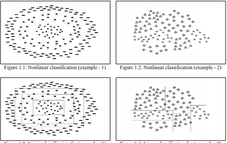
[image:16.595.85.527.447.726.2]To understand the motivation for using elliptical boundaries, consider Figures 1.1 and 1.2. It is clear that using linear classifiers as shown in Figure 1.3 and Figure 1.4 to solve such non-linear classification problems are not the suitable and appropriate solutions.
Figure 1.1: Nonlinear classification (example - 1) Figure 1.2: Nonlinear classification (example - 2)
4 Instead of the above boundaries, Figures 1.5 and 1.6 show the elliptical nonlinear boundaries which are more appropriate visually.
Figure 1.5: Elliptical classification for (example - 1) Figure 1.6: Elliptical classification for (example - 2)
1.3 Problem Definition
Given the motivation provided in the previous section, the problem is to develop a cost-sensitive decision tree algorithm with the following properties:
The algorithm should be suitable for multiclass problems. For example, in an application involving credit assessment, the task could involve constructing a classifier that predicts whether a customer is low, medium, high or very high risk.
The algorithm should take account of costs of different misclassification cases. For example, when dealing with fraud detection related to granting loans, the costs should not only be based on the true and false predictions (fraud / non-fraud) but also should consider the different amount of cost involved in each misclassification case.
The algorithm should be able to learn non-linear boundaries that reflect the data.
The algorithm should reduce the size of decision trees to make them easy to understand and interpret.
1.4 Aims and Objectives
5 misclassification cost and producing smaller decision trees that are easier to interpret and understand.
In order to achieve this aim, the following objectives are developed:
1- To conduct a deep survey of the field of cost-sensitive classification, in order to identify the strengths and weaknesses of existing approaches to cost-sensitive classification and problems faced by researchers addressing similar problems.
2- To develop and implement the proposed new algorithm (ECSDT) that could make a step forward in enhancing the performance of cost-sensitive classifiers.
3- To utilize and explore the performance of different evolutionary optimization methods such as Genetic Algorithms (GAs) and particle swarm optimization (PSO) during the implementation of the new algorithm (ECSDT).
4- To compare the results obtained by the new algorithm (ECSDT) against some common accuracy-based classifiers and some cost-sensitive decision tree methods available in the Weka system (Witten et al. 2016) such as J48 that implements the standard C4.5 algorithm (Hormann 1962), NBTree (Kohavi 1996), MetaCost (Domingos 1999) and CostSensitiveClassifier (Witten et al. 2016).
1.5 Research Methodology
This section describes the rationale for the particular research methodology adopted for this study.
Creswell (2003) defines research methodology as “a strategy or plan of action that links methods to outcomes, and it governs our choice and use of methods (e.g., experimental research,surveyresearch,ethnography,etc.)”.Researchmethodologydescribesthewaythat will be followed towards solving the research problem. It shows the various steps that are generally adopted by a researcher in studying his research problem along with the logic behind them (Kothari 2009). Any research should be planned and conducted based on what will best help to answer its research questions. There are three major types of methodologies that can be adopted when conducting research (Barks, 1995; Kraska, 2010):
6 Mixed research, which involves the mixing of quantitative and qualitative methods or
other paradigm characteristics.
1.5.1 Quantitative Research Methodology
The literature provides many definitions of a quantitative research methodology and the majority of them share the core principles. The quantitative research methodology can be defined as:
“Explainingphenomena by collecting numerical data that are analyzed using mathematically based methods (in particular statistics) ”(Sibanda 2009).
This definition describes clearly that quantitative methods are used to solve or explain problems by gathering the required numerical data and then applying mathematical and statistical methods to verify claims and hypothesis, such as whether one algorithm performs better than another.
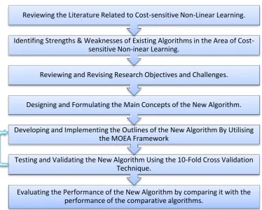
7 Figure 1.7: Methodology stages
The exploration activity firstly was mainly on handcrafted data where the best results are known and then extended for a number of real datasets from the UCI repository (Lichman 2013). When the exploration was over, the performance of the algorithm was evaluated against some of the well-known algorithms in this area. The empirical evaluation was done using a 10 fold cross validation methodology (Mudry & Tjellström 2011). The measures used are consistent with those widely used in the field, namely accuracy and cost of misclassification (Turney 1995). Since one of the main objectives of developing the new algorithm is to reduce the size of the decision trees, so, the size of the produced decision trees has been adopted as another criterion for the comparison. A wide range of datasets was used from the UCI repository (Lichman 2013) and the results are compared with the current state of the art in the field including algorithms such as those available in WEKA.
Evaluating the Performance of the New Algorithm by comparing it with the performance of the comparative algorithms.
Testing and Validating the New Algorithm Using the 10-Fold Cross Validation Technique.
Developing and Implementing the Outlines of the New Algorithm By Utilising the MOEA Framework
Designing and Formulating the Main Concepts of the New Algorithm. Reviewing and Revising Research Objectives and Challenges.
Identifing Strengths & Weaknesses of Existing Algorithms in the Area of Cost-sensitive Non-inear Learning.
8 1.6 Research Contributions
The main contributions of this research are:
Identifying weaknesses and strengths of the current algorithms in the field of cost-sensitive classification.
Developing and introducing a novel non-linear method (ellipses) to separate classes. Introducing a direct solution to multiclass classification problems without the need for dividing the multiclass problem into binary sub-problems as is the case with other algorithms when dealing with multiclass problems.
Exploring the performance of the new algorithm (ECSDT) when two different evolutionary optimization methods (PSO and GA) are applied and then comparing the results of the two methods.
1.7 Outline of Thesis
This PhD research is organized as follows.
Chapter 1 presents the general introduction to the research. This chapter sets out the motivation, problem definition, aims and objectives, research methodology, main contributions, and ends up with the outline of the thesis.
Chapter 2 contains two main sub-sections, the first sub-section presents the background for supervised learning and the second section presents the background for decision trees learning as they are both quite relevant to the area of research. The first sub-section presents, the main concepts of supervised learning, and gives some details on cross-validation techniques which are the most widely used methods for validating classification algorithms. The second sub-section provides a background on decision tree learning, gives some details about different feature selection methods that are adopted by different decision tree learning algorithms, and ends up with explanations of some measures that are adopted for evaluating the performance of decision tree algorithms.
9 are presented, different attempts and studies for inducing non-linear decision trees are presented, previous methods adopted for multiclass classification problems are illustrated, and ends up with a literature review about using evolutionary optimization methods such as GAs and PSO for inducing decision trees.
Chapter 4 describes the methodology adopted for developing the new algorithm, explains how ellipses are used to formulate cost-sensitive learning as an optimization problem, shows how ellipses are used to construct the decision tree, gives some explanations about the MOEA framework and how it is utilized for the implementation of the new algorithm and ends up with some illustrative examples of how the new algorithm works.
Chapter 5 provides some details about the datasets used for the empirical evaluation as well as some details about the comparative algorithms used to evaluate the performance of the new algorithm. This chapter also displays and discusses the results obtained when applying the three different implementations of the new algorithm (Accuracy only, cost only, and accuracy with cost) as well as comparisons of the obtained results with other algorithms.
10
Chapter 2
: GENERAL BACKGROUNDS
As mentioned in the introduction, this research aims for developing a new algorithm to induce cost-sensitive decision trees. As it is known, Decision tree learning is a supervised learning method, so that, this chapter firstly presents some relevant background on supervised learning which one of the main is fields of machine learning and then gives a general background on decision tree learning. Section 2.1 starts with a general background on the supervised learning field, and then explains the related basic concepts and terminology used in this field, after that lists the general steps for developing any supervised learning algorithm, and finally ends up with some detailed explanation about the Cross-Validation technique which is one of the most important techniques used in the development of the supervised learning algorithms. Section 2.2 gives a general background on decision tree learning and also provides some details on two very important topics related to learning decision trees. The first topic presents some details on the common methods used for feature selection when constructing decision tree algorithms and the second topic covers the common measures used for evaluating the performance of decision tree algorithms. Section 2.3 presents two important concepts that should be considered when building cost-sensitive classifiers, namely: a confusion matrix and a cost matrix.
2.1 Background of Supervised Learning
11 During the learning process adopted by machine learning algorithms, the learner interacts with the environment. Hence, the learning process may be explained as a means of using the experience to acquire skills and knowledge. The kind of interactions that are adopted by the machine learning algorithms during the learning process can help in grouping and categorize the learning processes into several categories. The distinction between supervised, semi-supervised and unsemi-supervised learning is observed quite frequently.
Supervised Learning: In this category, the classes in which the data elements were classified accordingly are well-known and clear, and there are well-specified boundaries for each class in a particular (training) data set, and the learning process will be accomplished using these classes (Suthaharan 2016). Every example (element) in supervised learning is a pair that involves an input feature(s) and a required output value. The training data is interpreted and evaluated by a supervised learning algorithm, which tries to determine how the input factors are related to the target factors. After this, an inferred function is created, known as a classifier model or a regression model. It is important that the produced model provides the correct output value for any new, valid, unobserved input element (Kotsiantis 2007). More details about supervised learning are given in section 2.1.
Unsupervised Learning: Unsupervised learning involves deducing and distinguishing different patterns in a particular dataset without knowing the class labels of any of the instances belonging to the dataset. With unsupervised learning, input data is processed by the learner to generate a summary or any targeted form of the data. A common example of this kind of learning is clustering in which a data set is clustered into subsets which have similarities in the targeted characteristics (Shalev-Shwartz & Ben-David 2014). Another example of unsupervised learning is the association rules techniques. Association rule learning is used to find suitable rules that can characterise a large part of the dataset, such as the customers that buy an X extra of goods whenever they aim to buy Y goods (Oellrich et al. 2014).
12 testing the unlabeled data on the model to set predicted class-labels for them and then a new supervised model is constructed using all the data which consists of the actually labeled data with the unlabeled data that have been given a predicted class-label (Board & Pitt 1989).
2.1.1 Basic Concepts of Supervised Learning
In supervised learning, some data obtained from a particular domain is used by the learning algorithmasaninput,andthenamodelbasedonthedomain’sstructureiscreatedasan output. That is, a model of the domain is created using a particular set of observations. The observations, on their own, are referred to as “instances” or “examples”, while a set of observationsisreferredtoasa“dataset”.Ineveryinstance,thereisasetofvaluesknownas the instance’s “attributes”.Foreachdataset,thesamegroup of attributes is used to define every instance. It is assumed by the majority of the applications of machine learning algorithms that the attributes may be of type “nominal” or of type “numeric”. Nominal attributes involve a set of unordered values, such as a set of colours {red, blue, green, etc.}, or a set of weather conditions {clear, rainy, windy, etc.}. Numeric attributes, in contrast, are either integers or real numbers. The space of every possible mix of attribute values is referred toas“instancespace”.
Decisiontreesarepartofmachinelearningmodelsthatareknownas“classifiers”.Classifiers aim to solve classification problems in which each instance of the dataset is labelled with a nominal attribute value knownasthe“actualclass”.Theinstancespaceisseparatedbythe classifier into several separated sub-spaces, and then one class is allocated to every sub-space. That is, it is presumed that every instance in the instance space is tagged with one nominal attributevalue,knownasthe“predictedclass”oftheinstance.
13 training instances. In a perfect situation, the classifier will help in classifying all the examples correctly.
When an instance is allocated the wrong class, then we refer to itasa“misclassified”instance or example. The predictive performance of a particular classifier is determined by its “accuracy”orbyits“errorrate”,andtheseshouldbedeterminedusinganindependentsetof labelled instances which are not used with the learning algorithm when it creates the classifier. This set of instances is referredtoas“testingdata”.The noise that is caused by allocating “incorrect”classlabelstotraininginstancesmaymisguidethelearningalgorithm.Thisissue arises as the learning algorithm builds a classifier in accordance with the class labels from the training data. Therefore, instances which are not labelled correctly need to be determined and it should be made certain that they have no impact on the construction of the classifier. When there is a close fit between the classifier and the training instances, then noisy instances may also fit with the classifier, making it a less valuable classifier. This problem is referred to as “overfitting”andausualtechniqueindecisiontreesistoremovethosepartsofaclassifierthat may overfit thetrainingdata.Thisprocess,knownas“pruning”andithelpsinincreasingthe accuracy as well as the comprehensibility of the induced classifier and also decreases the size of the classifier.
2.1.2 Developing Supervised Learning Algorithms
According to (Suthaharan 2016), four key stages should be followed to create a new supervised learning algorithm. These are training, testing, validation and evaluation, and are explained as follows:
14 1. Data domain extraction: This step involves extracting the data domain that has been formed by the feature space from the given data set. This is done to compute the required statistical measures and the variance among the feature space variables.
2. Response set extraction: The training data are provided with class labels, and hence, the labels of every observation can be extracted to develop some response sets that allow each data domains to be assigned to a particular response set. This set helps in computing the accuracy of the prediction and the prediction error by using the predicted responses extracted by the model and by its parameters.
3. Modelling: It refers to creating a relationship between the different variables. 4. Using class labels: The model training is a supervised learning approach; therefore, it is assumed that each instance of the training data has properly labelled with the proper class. If the labelling of the classes is not done properly, the training data considered as an invalid data because the accuracy of the prediction will be calculated as a ratio between the predicted class labels and the actual class labels for the dataset.
5. Optimization: This step includes updating the values of the parameters so that most of the computed responses are closer and corresponding to the actual class labels. This can be done using some quantitative measures, like distance measures and probabilistic measures (entropy and information gain).
Testing Phase: Model testing is a process that includes analyzing the efficiency of the model trained by the algorithm. That is, it will be confirmed through the testing phase is that the trained model also works on different labelled dataset called (testing dataset) that is not used during the construction of the model. Majority of the steps of the training phase are also part of the testing phase, with the only distinction being that in the training phase, is that the steps are repeated so that the optimal parameters can be obtained; however, in the testing phase, these steps are performed only once.
15 most common techniques used for the purpose of validation is the cross-validation method (Arlot & Celisse 2010). Through this validation, it is made certain that the overall dataset is completely trained, validated and tested so that the classification error can be minimized, and the accuracy can be maximized for the unseen data.
Evaluation Phase: In the evaluation phase, it is determined whether the trained and cross-validated model is useful when a different data set is used, that had not been used earlier in the training or validation phases. The labelled data set is only used in this phase to test the results given by the final model with respect to some evaluation metrics, like classification accuracy and execution time. For this purpose, there are various measures known as qualitative measures as they can determine the quality of the performance of the trained model. The measures that are often used include accuracy, specificity, sensitivity and precision, as described in (Costa et al. 2007).
2.1.3 Cross-Validation
The purpose of cross-validation was to solve the problem of overoptimistic outcomes given by training an algorithm and evaluating its statistical performance on the same data set (Suthaharan 2016). It was asserted earlier that the cross-validation technique is the most widely used method for validating classification algorithms (Arlot & Celisse 2010). It is shown in machine learning literature that there are different methods used for cross-validation. The most widely used cross-validation methods are presented and discussed in the following sub-sections.
16 following equation can be used to obtain the average accuracy for the K testing folds:
Average Accuracy =K1∑Ki=1Accuracy of Testing Fold[i]
2.1Here, K refers to the number of testing folds. By applying the K-Fold Cross-Validation it can be made sure that all observations are used for training and validation, and every observation is used just once for validation (Anguita et al. 2012)
Leave-One-Out: This method is a special case of K-fold cross-validation, where K refers to the number of instances in the dataset. In every iteration, the entire data except a single observation is used for training the model, and testing the model takes place on that single eliminated observation (Arlot & Celisse 2010). It is found that the accuracy measure attained using this approach is almost unbiased; however, there is a high variance, which leads to unreliable results (Arlot & Celisse 2010). Despite those shortcomings, this method is still used on a wide scale when the data is quite rare, particularly in bioinformatics that has limited quantities of data samples.
Leave-P-Out: In this approach, the testing set contains a number equals to P instances from a dataset contains N instances, while the remaining (N-P) are used as training, and this procedure is repeated for all possible combinations from the N instances (Celisse & Robin 2008). This cross-validation method is quite expensive to use due to the long computation time it consumes (Arlot & Celisse 2010).
Random Subsampling: In this method, K data splits of the dataset are carried out. In each split, a fixed number of examples are chosen without replacement as a testing set and the remaining examples considered as the training set. In each data split, retraining of the model takes place from the scratch with the training examples, and estimation is computed using the testing examples. Then the average of the different estimates is the final estimate obtained (Steyerberg et al. 2001; Kohavi 1995).
17 major and direct impact on the accuracy of the classification, as well as the computational complexity. It was mentioned by (Suthaharan 2016) that it is still quite difficult to divide datasets for training, validation and testing effectively, and no ideal method exists that can provide an optimal ratio for splitting the dataset.
2.2 Background of Decision Tree Learning
The purpose of data mining is to obtain valuable information from large datasets and to present it through illustrations that are easy to understand. One of the most successful methods of data mining is the decision tree that was initially presented in the 1960s. There is widespread use of decision trees in various fields (Song & Lu 2015). The main motivation to use a decision tree as the most widely used classifiers in the machine learning applications is that it can be used and understood easily.
According to the description given in (Song & Lu 2015; Olivas 2007; Rokach & Maimon 2005), a decision tree is a classifier that is presented as a recursive separation of the instance space. Therearethreekindsofnodesinthedecisiontree.Thefirstnodeisthe“rootnode”, which is an independent node that is not generated by any other node. All other nodes of the decision tree (except the root node), they should be branched off from another node. A node which has outgoing branches is referred to as a test or decision node. The other nodes which are not split any more are all known as leaves or end nodes.
In (Mitchell 1999; Song & Lu 2015; Olivas 2007; Tan et al. 2006), the way DT algorithms like ID3 (Quinlan 1986), C4.5 (Hormann 1962) and CART (Steinberg 2009)construct classifier models is explained, where every test node, including the root node, divides the instance space into two or greater sub-spaces consistent with a particular discrete function. Every leaf node is allocated to one class, which signifies the most widely occurring value. The new unseen instances are then labelled by passing them downwards from the root of the tree to a leaf, in accordance to the outcome ofthetestscarriedoutoverthepath,andconsideringtheleaf’s class label as the prediction class for the new unseen instance.
18 partially or entirely unnecessary or repetitive with respect to the target concept. It has been found in (Tang et al. 2014; Tan et al. 2006) that the efficiency, as well as the accuracy of the constructed decision trees, is influenced by the usage of some techniques that select only the most important features among others when developing DTs. This is because the aim of these methods is to select a small subset of the most influential features and removing the unnecessary ones in accordance with a particular evaluation criterion, leading to an improved learning performance (e.g., higher learning accuracy for classification, lower computational cost, lower running time for learning the algorithms, and better model interpretability).
Four main steps were presented by (Dash, Manoranjan and Liu 1997; Kumar 2014) to be followed in a standard feature selection method. These include:
Choosing the feature subset by making use of one the appropriate techniques, like the complete approach, the random approach or the heuristic approach (Muni et al. 2006);
Analyzing and evaluating the subset being chosen to determine and assess the discriminating capability of the selected feature or subset of features so that the various class labels can be identified and distinguished;
Defining the stopping criterion so that it can be determined when the feature selection process should be stopped from operating continuously in the space of subsets. Some of the common stopping criteria are given in (Rokach & Maimon 2005), and are listed as the following conditions:
1. When all instances in the training set are related to a single class. 2. When the predefined highest tree depth has been attained.
3. If the node were split, then the number of instances in one or more child nodes would be lower than the minimum number of instances permitted for child nodes. 4. When the value of applying the splitting criteria is not better than the specific predefined threshold.
Validating the outcomes so that the validity of the chosen subset can be tested by performing various tests, and then contrasting the findings with the results obtained previously.
19 2.2.1 Feature Selection Methods for Decision Trees
As demonstrated earlier, a decision tree is developed top-down from a root node and consists of dividing the data into appropriate subsets. Therefore, a significant query that arises is that “whichmeasureisthemostappropriateforchoosingthefeatureorsub-features that are most useful for dividing or categorizing a specified dataset”. Several algorithms have been described in the past studies that make use of various techniques for choosing the best features for dividing the dataset in every decision node when building decision trees. Brief descriptions are presented in the following paragraphs which highlight some feature selection techniques that have been used in the most common decision tree algorithms, i.e. CART, ID3 and C4.5.
GINI Index - CART
The CART algorithm was developed by Breiman in 1984. CART is an abbreviation that stands for Classification And Regression Trees.
Decision trees constructed using the CART algorithm are usually binary decision trees, that is, every split relies on the value of a single predictor variable, and there will be only two child nodes of every parent node. The splitting selection criterion that is used by CART is based on what is known as the GINI index. For any training set S, the following equation is used to compute the GINI index of S (Gupta & Ghose 2015):
𝐺𝑖𝑛𝑖 (𝑆) = 1 − ∑𝑘𝑖=1𝑝𝑖2 2.2
Where (k) refers to the number of class labels, Pi refers to the probability that an instance in S is part of the class (i).
The GINI index for choosing the attributes A in the training dataset (S) is subsequently described as follows:
Gini (A, S) = Gini (S) – Gini (A, S)
= Gini ( S) − ∑ | 𝑆𝑖 |
| 𝑆 | 𝑛
20 Entropy and Information Gain - ID3
ID3 is an abbreviation of (Iternative Dichotomizer 3), which is an entropy-based algorithm, where the split criterion is developed such that it seeks an improvement in the purity of leaves (Quinlan 1986). The basis of this criterion is the information theory, and the feature having the largest information gain is given preference. Information gain seeks to measure how well a specific feature sets apart the training examples on the basis of their target classification (Ballester & Mitchell 2010). The entropy that the ID3 algorithm adopts initially was based on the entropy concept discovered by Claude E. Shannon in (Shannon 1948) that computes the sample’shomogeneity.Whenthesampleis fully homogeneous, then the entropy is zero, and when the sample is equally divided, then there is entropy of one. Hence, the ideal choice for splitting is the feature that has the higher decrease in entropy (Peng et al. 2009).
Shannon’sentropy(Shannon 1948) for an attribute A is described as follows:
E(A) = − ∑ (pni=1 i log2 pi) 2.4
Here, (n) refers to the number of classes, and (pi) is the probability of examples that are part of the class (i) in the set.
Information gain is an add-on to the entropy concept and explains the significance of a specified attribute A of the feature vectors. It is also used to determine the way the more informative attributes are ordered in the nodes of a decision tree. The information gain for an attribute A in a given dataset S determines the variation in entropy from prior to and following the splitting of the training set S on the attribute A. The following equation can be used to calculate this information gain:
IG (S, A) = E (S) – E (A) 2.5
Here, E(S) refers to the entropy of the present training set prior to the splitting. The concept of developing a decision tree is based on determining the attribute that offers the largest information gain.
Gain Ratio - C4.5
The C4.5 algorithm is an extension to the ID3 algorithm, both of which have been designed by Quinlan.
21
Continuous and discrete features are both approved.
Incomplete data points are managed.
The issue of over-fitting is resolved by adopting the bottom-up method, which is referredtoas“pruning”.
One of the two given criteria can be adopted by C4.5. The First criterion is the information gain explained in the preceding section. The second criterion is an entropy-based criterion that is also based on the information gain. Information gain was found to show a preference for attributes that had a high degree of cardinality (having a large number of potential values). The ideal variable for splitting is one that is unique for every record. C4.5 computes the possible information from each partition (highest possible information) and contrasts it with the actual information. This is referred to as the Gain Ratio. Normalization to information gain is applied by the Gain Ratio, where a value defined as follows is used:
SplitInfoA(S) = − ∑𝑣𝑖=1(|𝑆𝑖| / |𝑆|) log2(|𝑆𝑖| / |𝑆|) 2.6
This value is indicative of the information produced by splitting the training dataset S into v partitions according to v results of a test on the attribute A. The gain ratio is subsequently explained as follows:
Gain Ratio (A) = Information Gain (A) / SplitInfoA(S)
2.7 Here, IG (A) refers to the information gain for choosing attribute A and is computed as depicted in section (2.1.2.2). Once the Gain Ratio for every attribute is determined, the attribute having the largest gain ratio is chosen as the splitting attribute.2.2.2 DTs Performance Measures
(Osei-22 Bryson 2004). The most widely used performance criterion for assessing machine learning algorithms are presented in the following sub-sections.
2.2.2.1 Statistical Measurements
The literature of machine learning shows that various statistical performance tools were used to statistically analyze the efficiency of machine learning algorithms. The most widely used methods for this purpose are an Error rate, Accuracy Rate, Precision, Recall and F1-Score etc. A brief explanation of these evaluation metrics and how they are calculated are given in the following short paragraphs (Fawcett 2006; Powers 2011; Alvarez 2002; Davis & Goadrich 2006).
Accuracy Rate: It refers to the ratio that is attained by dividing the number of accurate estimations with the overall number of estimations.
Accuracy =TP+TN+FP+FNTP+TN 2.8
Error Rate: It is the ratio of all estimations that are not correct. It basically measures how inaccurate a model is.
Error =FP+FN+TP+TNFP+FN 2.9
Precision Rate: It refers to the number of positive predictions divided by the overall number of positive class values estimated. That is, it is the ratio of True Positives to the overall number of True Positives as well as the number of False Positives. This is also referred to as the Positive Predictive Value (PPV).
Precision (PPV) = TP+FPTP 2.10
Recall Rate: It is the ratio of True Positives to the number of both True Positives and False Negatives. That is, it is the ratio of the positive estimations to the number of positive class values in the testing data. This ratio is also referred to as the Sensitivity or the True Positive Rate.
Recall =TP+FNTP 2.11
23
F1 − Score = 2 ∗Precision+RecallPrecision∗Recall 2.12
2.2.2.2 DT Comprehensibility
Decision trees are usually considered to be the most precise and efficient classification methods, however, at times, DTs, particularly the bigger ones, are difficult to comprehend and explain. Therefore, they become incomprehensible to experts (J.R. Quinlan 1987), so it is vital to make sure that DTs are as easy to understand so that they can be interpreted even by non-professionals. The complexity of DT is normally measured using one of the metrics given below (Olivas 2007):
The numbers of nodes that create and construct the tree.
The number of leaves that are created by the tree
The tree depth, i.e. the length of the largest path, from a root to the leaf, and a total number of attributes considered.
Various techniques have been presented in the last few years to simplify trees. These include pruning methods that are possibly the methods used most extensively to decrease the size of DTs. In machine learning, pruning is the process of removing non-predictive subtrees (branches) of a model so that its accuracy can be increased, size can be decreased, and the issue of overfitting can be avoided (Patel & Upadhyay 2012). Pruning is of two kinds, pre-pruning and post-pre-pruning (Fürnkranz 1997). Pre-pre-pruning is also known as forward pre-pruning, which prevents the growth of trees early on, at the beginning of the process of constructing the DTs, so that the generation of unimportant branches can be avoided. Post-pruning is also known as backward pruning. In this method, the tree is first constructed and then, the unimportant branches of the decision trees are reduced.
24
2.2.2.3 Stability of the Results
Another important factor to consider when creating and assessing the efficiency of DTs is the stability of the DT prediction findings. The criterion of stability performance is important with respect to the quality of DT, as there should not be much difference in the predictive accuracy rate when a DT is used on various validation data sets (Osei-Bryson 2004). One of the most widely used methods by the developers is the k-fold cross-validation estimator (particularly when there is a limited amount of data) which helps to make sure that the outcomes attained by the various DTs are constant and also help in providing an optimal decrease in variance (Kale et al. 2011). More details on K-fold cross-validation is given before in section 2.1.3.
2.3 Confusion and Cost Matrices
To take account of misclassification costs, there are two important concepts that should be considered when building the classifier, namely: a confusion matrix and a cost matrix, which are introduced below.
25 Confusion Matrix Predicted Class
Pos (+) Neg (-) Actual Class Pos (+) TP FN
Neg (-) FP TN
Table 2.1: The confusing matrix for binary classification problem
Cost Matrix Predicted Class Pos (+) Neg (-) Actual Class Pos (+) C (+,+) C (+,-) Neg (-) C (-,+) C (-,-) Table 2.2: The cost matrix for binary
classification problem
The ordinary binary confusion and cost matrixes described above can be extended to multiclass problems. For example Tables 2.3 and Table 2.4 respectively give the forms of a confusion matrix and a cost matrix for a problem labelled with three classes (A, B and C) wherein the confusion matrix: AA denotes the number of examples that are actually of class A and predicted as class A. AB denotes the number of examples that are actually of class A and predicted as class B and so on for the rest. And for the cost matrix C(AA) denotes the cost of (AA), C (AB) denotes the cost of misclassifying A as B and so on for the rest.
Confusion matrix
Predicted Class
A B C
Actual Class
A AA AB AC
B BA BB BC
C CA CB CC
Table 2.3: The confusion matrix for a 3-classes classification problem
Cost matrix
Predicted Class
A B C
Actual Class
A C(AA) C(AB) C(AC) B C(BA) C(BB) C(BC) C C(CA) C(CB) C(CC) Table 2.4: The cost matrix for a 3-classes
classification problem
Elkan (Elkan 2001) and Ling & Sheng (2008) described how important it is to consider the misclassification costs in various cost-sensitive learning algorithms and mentioned that, when the cost matrix is defined, a new instance x should be classified into the class (i) that leads to the minimum expected cost L(x, i) which is expressed as:
L(x, i) = ∑nj=1p(j | x) ∗ c (i, j) 2.13
Where p ( j | x ) is the probability of classifying an instance x into class j, and c (i, j ) is the cost of predicting class (i) when the true class is j.
26 Accuracy Rate = ∑ 𝑻𝑪𝒊
𝒎 𝒊=𝟏
𝑵
2.14 Where m is the number of class-labels the dataset has, 𝑇𝐶𝑖 is the number of examples of Class C that have been classified correctly and N is the total number of examples. Then the accuracy rate for the confusion matrix depicted in Table 1.1 can be as the following form:
Accuracy Rate = (AA +BB+ CC) / N where, N is the total number of examples.
Error Rate = ∑ 𝑭𝑪𝒊
𝒎 𝒊=𝟏
𝑵
2.15 Where m is the number of class-labels the dataset has, 𝐹𝐶𝑖 is the number of examples of Class C that have been classified incorrectly and N is the total number of examples. Then the error rate for the confusion matrix depicted in Table (1.1) can be as the following form:
Error Rate = (AB+ AC+ BA+ BC+ CA+ CB) / N where, N is the total number of examples.
The error rate can also be calculated as a complement to the accuracy rate, then Error Rate = 1 - Accuracy Rate 2.16
Utilising the confusion matrix in Table 1.1 and the cost matrix in Table 1.2, we can calculate the total misclassification cost for the classifier using the Eq 1.1 as follows: Total Cost = AA*C(AA) + AB*C(AB) + AC*C(AC) + BA*C(BA) + BB*C(BB) + …………
To illustrate the ideas in an applied manner, suppose that we have a multiclass problem with the following confusion and cost matrixes shown in Tables 2.5 and 2.6 respectively.
Confusion matrix
Predicted Class
A B C
Actual Class
A 50 0 0
B 0 45 5
C 0 5 45
Table 2.5: Confusion matrix (Example-1)
Cost matrix Predicted Class
A B C
Actual Class
A 0 5 5
B 5 -5 50
C 50 100 0
27 Then,
Accuracy Rate = (50+45+45) / 150 = 0.9333 = 93.33 % Error Rate = (5+5) / 150 = 0.0666 = 6.66 %
Also the Error Rate can be calculated a complement to the Accuracy Rate as following: Error Rate = (1 - 0.9333 = 0.0666 = 6.66 %)
The Total Cost = (0* 50) + (5*0) + (5*0) + (5*0) + (-5*45) + (50*5) + (50*0) + (100*5) + (0*45) = 525 units of cost.
As we notice from the cost matrix above, the cost of BB is (-5), and this is allowed as (Turney 1995) mentioned that assigning negative costs for classification can be interpreted as benefits. As a second example to illustrate the cost vs accuracy issue, using the same cost matrix shown in Table 2.6, consider a situation where another different algorithm is applied and results in the following confusion matrix:
Confusion matrix
Predicted Class
A B C
Actual Class
A 50 0 0
B 10 40 0
C 10 0 40
Table 2.7: Confusion matrix (Example-2) Then,
Accuracy Rate = (50+40+40) / 150 = 0.8666 = 86.66 % Error Rate = (1 - 0.8666 = 0.1334 = 13.34 %)
The Total Cost = (0* 50) + (5*0) + (5*0) + (5*10) + (-5*40) + (50*0) + (50*10) + (100*0) + (0*40) = 350 units of cost.
28
Chapter 3
: THE LITERATURE REVIEW
Considering that the main objective of this research is the development of a new nonlinear cost-sensitive decision tree for multiclass problems by utilizing some multi-objective optimization methods, this chapter presents a review of the literature that covers four related areas Cost-Sensitive Decision Trees, Nonlinear Classification, Multiclass Classification and Multi-Objective Optimization. Section 3.1 starts by reviewing the general literature on cost-sensitive learning and then gives some explanations on cost-cost-sensitive strategies, after that, the categories of cost-sensitive algorithms according to the method adopted for implying the cost were presented, and finally, a more detailed literature on cost-sensitive decision trees which is at the core of this research is presented. Section 3.2 covers nonlinear decision tree. Section 3.3 presents some literature on multiclass classification, and Section 3.4 presents the field of multi-objective optimization using PSO and GAs.
3.1 Cost-Sensitive Learning
The literature on classification in data mining and machine learning shows that many approaches have been developed for data classification, including decision trees, Bayesian networks, neural networks, discriminant analysis, and support vector machines, among many others (Freitas et al. 2009).
Prior to the emergence of cost-sensitive classification algorithms, the classification systems in the past only aim to enhance the classification and prediction accuracy for the classification system (Ling & Sheng 2008). Hence, in the previous decades, the cost-sensitive classification was considered to be an important topic to attract the attention of the researchers in the field of data mining and machine learning which led to the development of many methods and algorithms that take into account the costs when performing the classification (Lomax & Vadera 2011; Turney 1995).
cost-29 sensitive learning techniques focus on those applications in which misclassification errors consist of various costs, and where some of the misclassification errors are more costly compared to others. In a medical diagnosis, for instance, an ill patient who is categorized as healthy is considered as a more expensive error (which can cause a loss of life) compared to categorizing a healthy patient as a sick one (which may merely require additional tests). Another example is when a company issues a credit card to a customer where the loss is normally costlier than an error of refusing a credit card to a good client (Jin Li et al. 2005).
A taxonomy of various costs in learning classification problems has been presented by (Turney 2002). These include costs of testing, costs for misclassification errors, costs of interventions, costs of computation, costs of unwanted achievements, costs of instability, and costs of human-computer interaction.
3.1.1 Cost-Sensitive Learning Theories and Strategies
With cost-sensitive learning, the new example that is to be classified should be labelled with the class that leads to the lowest expected cost and the literature shows many attempts introduced by several authors to formalize the cost-sensitive learning problem (Elkan 2001; Turney 1995). These formulations are based on computing the cost of classification using a confusion matrix and a cost matrix.
30 Another attempt for categorizing cost-sensitive learning algorithms is that presented at the comprehensive survey carried out by Lomax and Vadera (Lomax & Vadera 2011) which listed several ways to categorize the algorithms intended for inducing cost-sensitive decision trees. They listed some of the algorithms that are distinct in accordance with the kind of cost(s) included. The purpose of some of these algorithms was to decrease just the misclassification costs; others aim to minimize only the cost of obtaining the information, whereas some others aim to decrease both previous expenses. Then, they categorized the cost-sensitive algorithms depending on the approach adopted. It was asserted by them that there are two key techniques that were used in algorithms to develop the cost-sensitive decision tree. The greedy method is used in the foremost category, where a single tree is developed at a time. The most famous algorithms that use the greedy approach are ID3 (Quinlan 1986) and CART (Breiman et a., 1984). The second category adopts the non-greedy approach that intended for inducing multiple trees.
In the following sub-sections, these categories will be discussed in some details. In section 3.1.1.1, Direct Cost-Sensitive Learning approaches will be described, section 3.1.1.2 gives some highlights related to the meta-learning cost-sensitive approaches. Since this research is about developing a new cost-sensitive decision tree algorithm, a separate sub-section 3.1.1.3 has been allocated to give some detailed explanation on some common Cost-Sensitive Decision Tree algorithms.
3.1.1.1 Direct Cost-Sensitive Learning
When constructing direct cost-sensitive learning algorithms, the key concept is to directly include and use misclassification costs or other kinds of costs while developing the learning algorithms. Various algorithms were depicted in the previous studies that adopt direct cost-sensitive learning techniques; one of the adopted methods is by changing cost-incost-sensitive algorithms like (decision trees, Naïve Bayes, Neural Networks and Support Vector Machine) into cost-sensitive ones by modifying and changing the algorithm itself so that it includes functions that include costs while building the classifier .