Flow duration curve integration into digital filtering algorithms for simulating climate variability based on river baseflow

Flow­duration curve integration into 

digital filtering algorithms for simulating 

climate variability based on river baseflow

Mohammed, R and Scholz, M

http://dx.doi.org/10.1080/02626667.2018.1519318

Title

Flow­duration curve integration into digital filtering algorithms for 

simulating climate variability based on river baseflow

Authors

Mohammed, R and Scholz, M

Type

Article

URL

This version is available at: http://usir.salford.ac.uk/id/eprint/48450/

Published Date

2018

USIR is a digital collection of the research output of the University of Salford. Where copyright 

permits, full text material held in the repository is made freely available online and can be read, 

downloaded and copied for non­commercial private study or research purposes. Please check the 

manuscript for any further copyright restrictions.

Full Terms & Conditions of access and use can be found at

http://www.tandfonline.com/action/journalInformation?journalCode=thsj20

Hydrological Sciences Journal

ISSN: 0262-6667 (Print) 2150-3435 (Online) Journal homepage: http://www.tandfonline.com/loi/thsj20

Flow–duration curve integration into digital

filtering algorithms for simulating climate

variability based on river baseflow

R. Mohammed & M. Scholz

To cite this article: R. Mohammed & M. Scholz (2018): Flow–duration curve integration into digital filtering algorithms for simulating climate variability based on river baseflow, Hydrological Sciences Journal, DOI: 10.1080/02626667.2018.1519318

To link to this article: https://doi.org/10.1080/02626667.2018.1519318

© 2018 The Author(s). Published by Informa UK Limited, trading as Taylor & Francis Group.

Accepted author version posted online: 10 Sep 2018.

Published online: 02 Oct 2018.

Submit your article to this journal

Article views: 67

Flow

–

duration curve integration into digital filtering algorithms for simulating

climate variability based on river baseflow

R. Mohammeda,b_{and M. Scholz}b,c,d

a_{Faculty of Engineering, University of Babylon, Al-Hilla, Iraq;}b_{Civil Engineering Research Group, School of Computing, Science and Engineering,} University of Salford, Greater Manchester, UK;c_{Division of Water Resources Engineering, Department of Building and Environmental Technology,} Faculty of Engineering, Lund University, Lund, Sweden;d_{Department of Civil Engineering Science, School of Civil Engineering and the Built} Environment, University of Johannesburg, Johannesburg, South Africa

ABSTRACT

A baseflow separation methodology combining the outcomes of the flow–duration curve and the digital filtering algorithms to cope with the restrictions of traditional procedures has been assessed. Using this methodology as well as the monitored and simulated hydro-climatological data, the baseflow annual variations due to climate change and human-induced activities were determined. The outcomes show that the long-term baseflow index at the upstream sub-basin is nearly half of that at the downstream from October to April, whereas they are close to each other for the remaining months. Some of the groundwater reacts to precipitation and an evident rise in the groundwater contribution was detected for the hydrological years 1998–2001 and 2006–2008. The contrary was recorded for1987. The water released from the reservoir in the dry periods led to distinctions in the detected baseflow index between the pre-damming and post-damming periods of the river.

ARTICLE HISTORY

Received 26 April 2018 Accepted 21 June 2018

EDITOR

A. Castellarin

ASSOCIATE EDITOR

A. Langousis

KEYWORDS

climate change;

groundwater involvement; hydro-climatology; influence of human activity; surface water; water resources management

1 Introduction

1.1 Context

Separation of the river flow hydrograph into baseflow and direct runoff is a valuable method to comprehend subsurface water contributions to a stream, particularly when dealing with various water resources regulation problems (Lu et al. 2015, Mohammed and Scholz

2016). These procedures have also been applied to calculate the subsurface water proportion of hydrolo-gical resources and to contribute to the estimation of recharge. The direct runoff element denotes the extra discharge contributed by groundwater and surface run-off. However, the baseflow element denotes constant groundwater flow additions to streamflow, which is often important for water resources assessments (Brodie and Hostetler2005).

The baseflow index (BFI) represents the ratio of the baseflow to the total flow and can be calculated by applying a hydrograph separation method. Generally, this index can vary from 0.15 to 0.20 for an imperme-able basin and be more than 0.95 for a large-capacity basin. The BFI relates to basin characteristics such as soil type, geology, topography, plants and regional cli-mate (WMO2009, Price2011).

Numerous procedures have been suggested for base-flow separation, which are usually classified into three main groups: graphical methods (Linsley et al. 1988), digital filtering algorithm frequency assessment, and recession analysis (Welderufael and Woyessa 2010, Mohammed and Scholz2016). Nathan and McMahon (1990) differentiated techniques for constant separation by various flow proportions (Tallaksen and van Lannen

2004). Graphical methods separate the flow hydro-graph by linking the intersecting point of the baseflow and the runoff on the bottom point at the rising limb of the flow hydrograph, where it is anticipated that all discharges are considered as baseflow (Linsley et al.

1988, Welderufael and Woyessa2010). These methods separate the baseflow by many techniques that differ in their complexity: constant flow rate, constant slope and concave techniques (Al-Faraj and Scholz 2014). Lim

et al. (2005) highlighted that the major disadvantage of the graphical procedures is the lack of reliable results, even for the same flow dataset.

The United Kingdom Institute of Hydrology (UKIH) method is applied for daily mean flow data and is founded on the identification and interpolation of turn-ing discharge values in a measured streamflow time series (Piggott et al. 2005). The turning points represent the

CONTACTM. Scholz [email protected]

© 2018 The Author(s). Published by Informa UK Limited, trading as Taylor & Francis Group.

time in days and equivalent discharge values, where the recorded streamflow value is anticipated to be the total baseflow. For turning point calculations, the flow values are divided into a series of 5-day parts, and the lowest values of flow within each part (anxandypair, wherexiis the day on which the lowest flow value ofyihappened)

are the turning points. Then, the candidate turning point is compared to the preceding and following parts. Turning points are tested using the condition 0.9 ×yi< min(yi_˗1,yi+1) (Piggottet al.2005). The baseflow

temporal variation is computed by piecewise linear inter-polation connected by sequential sets of turning points.

The digital filtering algorithm (DFA) is the most commonly utilized approach in streamflow separa-tion and divides the baseflow by a processing method (Welderufael and Woyessa 2010, Mohammed and Scholz 2016). This procedure can be automated (Eckhardt 2005, Mohammed and Scholz 2016). For the purpose of this paper, two DFAs were assessed: the Eckhardt (2005) and the frequently applied Chapman (1999) procedures.

The flow–duration curve (FDC) can be defined as a curve showing the percentage of time that a streamflow is likely to be equivalent to or greater than a specific value. This plot describes the cap-ability of the basin to provide flows of various magnitudes. The lower and upper parts of the plot profile are essential in evaluating the channel and basin attributes. The form of the high-flow area indicates the type of flood that the basin is describ-ing, while the form of the low-flow region charac-terizes the basin capacity to sustain low flow during the dry season. Generally, Q50 is taken to be the

median flow. A flow of ≥Q50 is understood to be

low flow (Welderufael and Woyessa 2010, Mohammed and Scholz 2016). The ratio Q90/Q50

(i.e. the ratio of recorded flow ≥90% and ≥50% of the time) denotes a percentage of the river flow subsurface water aquifer contribution, or the corre-sponding proportion of the baseflow component (Al-Faraj and Scholz 2014, Gordon et al. 2004, Stewart 2015).

The baseflow timing and quantity can be impacted by many factors, such as climate, human activities (e.g. river damming) and basin characteristics. Many scien-tists have analysed the baseflow contribution to stream-flow (e.g. Partingtonet al.2012, Fanet al.2013, Mei and Anagnostou 2015, Rumsey et al. 2015, Stewart 2015, Wanet al.2015, Heet al.2016, Lottet al.2016, Miller

et al. 2016, Mohammed and Scholz 2016). However, they have used and/or compared many traditional tech-niques without taking into consideration climate change, drought phenomena and/or human-induced activities.

To address the knowledge gap, this study considers such impacts on the baseflow of a stream.

1.2 Rationale, aim, objectives and importance

The impact of a combination of anthropogenic inter-vention and climate change on the streamflow of a basin differs subject to climatic zone arrangement. Consequently, this should be investigated at a local scale (e.g. basin or sub-basin). Recently, due to uni-versal climate variability and local human-induced stresses, many areas have been affected by floods and droughts. Thus, evaluating the impact of such changes is important for understanding the mechanisms of hydrological response at a basin scale, regional water resources organization and flood and drought protec-tion. The Lower Zab River Basin (LZRB) has witnessed substantial alterations in hydro-climatic variables, as well as human activities, in recent years. Accordingly, this basin can be considered as an excellent case study for evaluating the hydrological influence of climate variability and anthropogenic intervention.

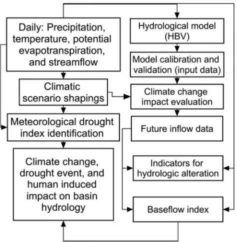
The aim of the current research was to apply the methodology of Mohammed and Scholz (2016) to assess the impact of climate change, drought events and human activities on the baseflow contribution to streamflow. In addition, multiple aspects of basin hydrology were addressed. This was accomplished by addressing the following objectives: (i) to investigate the spatio-temporal characteristics of meteorological data at monthly and annual time periods; (ii) to apply the approach developed by Mohammed and Scholz (2016) to study the effects of climate change, drought events and anthropogenic interventions on the base-flow of the LZRB (Fig. 1); (iii) to quantify the spatio-temporal baseflow contribution to the LZRB; and (iv) to analyse the sensitivity of the baseflow and reservoir inflow to the collective impact of climate change.

2 Materials and methodology

2.1 Illustrative case study area

The Lower (Lesser or Little) Zab River is a key stream of the Tigris River located near Erbil (northeastern Iraq). The watercourse system is located at latitude 36°50′N–35°20′N and longitude 43°25′E–45°50′E (Mohammed et al. 2018), as shown in Figure 1. The associated river basin is subject to a varied range of hydro-climatic conditions, as well as upstream and downstream structural improvements (Mohammed and Scholz 2017a). Accordingly, the basin has been selected as an illustrative case study for both semi-arid and semi-arid areas. The stream originates in the Zagros Mountains in Iran and flows approximately 370 km southeast and southwest through northwestern Iran and northern Iraq before joining the Tigris near Fatha city, which is situated approx. 220 km north of Baghdad (Mohammed and Scholz 2016), with a total distance of approximately 302 km. The river basin area is approximately 19 254 km2, of which nearly 76% is located in Iraq. The average yearly volume of the river at Dokan and Altun Kupri-Goma is about 6 × 109and 7.8 × 109 m3, respectively (Mohammed and Scholz

2017c) (Fig. 1). Dokan is the main dam that was con-structed within the upper part of the basin to control

the discharge of the river, store water for irrigation purposes and to provide hydro-electric power.

2.2 Meteorological drought identification

This study applied the reconnaissance drought index (RDI) for drought identification (Vangeliset al.2013). This index is founded on the relationship between the two aggregated quantities of precipitation and potential evapotranspiration (Tsakiris and Vangelis 2005). The RDI can be expressed in alpha (RDI_αk), normalized

(RDIn) and standard (RDIst) forms. The RDIst can be

applied for drought harshness calculations and the RDI_αk can be used as an index of aridity. A positive

RDIst indicates a wet period and a negative number

indicates a dry period compared to the natural regional conditions. The RDI_αkis usually estimated by:

RDI_αi

0¼ P12

j¼1Pij

P12

j¼1PETij

i¼1 toN andj¼1 to 12 (1)

where Pij and PETij are, respectively, the precipitation

and the potential evapotranspiration of thejth month and the ith hydrological year, which in Iraq starts in October, and N is the total number of hydrological years for the equivalent climate.

The values of RDI_αkare equal to both the lognormal

and the gamma distributions for many locations at various time periods (Tigkas 2008). By utilizing the gamma distribution, RDIstcan be estimated by:

RDIi_st ¼yiy

^

σ (2)

whereyi is ln(αki),ӯis its arithmetic average, andσy is the associated standard deviation.

Equation (3) can be applied for RDIstevaluation for

the gamma distribution (Tigkas2008):

g xð Þ ¼ 1

βγΓð Þγ xγ1e

x

β _forx >_{0 (3)}

whereγ,βandΓ(γ) are the shape, scale parameter and gamma function, respectively. The parametersγand β of the gamma probability distribution can be estimated by the following equations:

γ¼ 1

4A 1þ

ffiffiffiffiffiffiffiffiffiffiffiffiffiffi

1þ4A 3

r !

(4)

β¼x_γ (5)

A¼lnð Þ x

P

lnð Þx

N (6)

The drought severity rises when RDIstvalues are

mini-mum. The RDIst values can be categorized into eight

classes (Vangelis et al. 2013, Mohammed and Scholz

2017c), as shown inTable 1. For more details regarding

this index, readers are referred to earlier research stu-dies (Tigkaset al.2012, Mohammedet al.2017b).

2.3 Flow–duration curve and digital filtering algorithms

Daily flows at two key hydrological stations (Dokan and Altun Kupri-Goma Zerdela) were analysed by applying the methodology suggested by Mohammed and Scholz (2016). The Eckhardt (2005) approach was used to achieve low-pass filtering of the flow hydrograph to sepa-rate baseflow, which is mathematically expressed by:

BFt¼

1BFImax

ð Þ αBFt1þð1αÞ BFImaxTFt

1αBFImax

(7)

where BF (m3/s) is the separated baseflow, BFI is the baseflow index, TF (m3/s) is the total flow andαis the Eckhardt filter parameter, subject to BFt≤TFt.

Two parameters are needed for the Eckhardt recursive method identification (Eckhardt2005): (i) the recession constantα(Eckhardt parameter), which stems from the recession curve of the hydrograph valuation; and (ii) BFImax, which cannot be measured, but can be enhanced

based on the results of other methods. Eckhardt (2005) introduced three typical BFImaxvalues for diverse

hydro-logical and hydrogeohydro-logical environments: BFImax= 0.80

for perennial streams with porous aquifers, BFImax= 0.50

for ephemeral streams subjected to permeable aquifers, and BFImax= 0.25 for perennial streams with

imperme-able aquifers. As a first approximation, this study used BFImax= 0.25 (Eckhardt2005, Stewart2015).

Chapman (1999) discussed the second recursive DFA, which can be estimated by:

DFt¼

3α1

3α TFt1þ 2

3αðTFtTFt1Þ (8) where DF (m3/s) is the direct runoff, TF (m3/s) is the total flow,α is the filter parameter and tis the indivi-dual time step.

Based on the suggested approach, the outcomes of the FDC study were combined with the results from Equation (7) to gain anαvalue, considering BFImax= 0.25 (Eckhardt

2005) for perennial rivers with predominantly porous aquifers, as a first estimation. First of all, the long-term

Table 1.Drought classification based on the standardized reconnaissance drought index (RDIst) values.

No. RDIstrange Drought class No. RDIstrange Drought class

1 ≥2.0 Extremely wet 5 0.00 to−0.99 Near normal 2 1.99–1.50 Very wet 6 −1 to−1.49 Moderately dry 3 1.49–1.00 Moderately wet 7 −1.5 to−1.99 Severely dry 4 0.99–0.00 Normal 8 ≤ −2.0 Extremely dry

mean annual fraction of the total flow from the baseflow was estimated after obtaining the Q90and Q50values by

applying the FDC method, connecting Equation (7) with FDC (Al-Faraj and Scholz2014, Mohammed and Scholz

2016). Consideringα= 0.925 as an initial number (Arnold and Allen1999, Smakhtin2001), filtering of daily flow was undertaken for various values of the filter parameterαup to a point when the BFI was equivalent to the ratio Q90/

Q50. By applying the filteredα, several baseflow time series

could be gained. Secondly, linear regression models were performed between the annual BFI and the corresponding runoff for all considered periods at both the upstream and the downstream sub-basins to investigate climate change, drought events and river regulating impacts on the base-flow contribution (Mohammed and Scholz2016).

2.4 Data availability, collection and analysis

2.4.1 Meteorological data

Daily meteorological data, which included precipitation and minimum and maximum air temperature from 10 stations with elevations between 319 and 1536 m a.s.l., were gathered for the period 1979/80 to 2012/13 (Table 2 andFig. 1).

2.4.2 Hydrological data

The daily flow data were evaluated at two key hydrometric stations: Dokan (35°53′00″N; 44°58′00″E) and Altun Kupri-Goma Zerdela (35°45′41″N; 44°08′52″E). The drai-nage area for Dokan is estimated at 12 096 km2and data are available for the period 1931–2013, whereas the corre-sponding values for Altun Kupri-Goma Zerdela are 8509 km2and 1931–1993 (Mohammed and Scholz2017b).

2.4.3 Geospatial data

Iraqi boundaries and the LZRB shape files were down-loaded from the Global Administrative Areas (GADM

2012) and the Global and Land Cover Facility (GLCF

2015) databases, respectively. The GADM is a spatial database of the location of the world’s administrative areas (or administrative boundaries) for use in geo-graphic information system (GIS) and similar software. The GADM describes where these administrative areas are located and, for each area, provides some attributes such as the name and corresponding variant names, whereas the GLCF is a centre for land cover discipline, with a focus on study using remotely sensed satellite data and products to access land cover change for local, national and global systems.

For hydro-climatic stations, site projections, weighted average calculations and stream catchment outlines, ArcGIS 10.3 was used. Table 2 summarizes the location details of the meteorological stations. Statistical analyses, including the daily hydro-climatic datasets, comprising trend test, monthly and annual amounts, modifications and the filling of data gaps, were completed by the Statistical Program for Social Sciences (SPSS) (ITS 2016). The estimation of PET (mm) was performed by the FAO Penman-Monteith standard method (Allen et al. 1998) which was esti-mated based on the reference evapotranspiration, ETo

(mm), calculator version 3.2 (FAO,2012).

The weighting mean method was used for rainfall spatial distribution estimation. The process is often seen as essential for engineering praxis. For more infor-mation and detailed descriptions of this method, read-ers are referred to many previous studies, such as Mohammedet al. (2018).

The DrinC 1.5.73 software was used to calculate the RDIst values. The Indicators of Hydrologic Alteration

software (version IHA 7.1) (The Nature Conservancy

2009) was used to evaluate the natural flow regime alteration that resulted from climate change linked to human-induced activities. For flow–duration curve esti-mation and baseflow separation, HydroOffice (2015) for BFI+3.0 and FDC was used (https://hydrooffice.org/

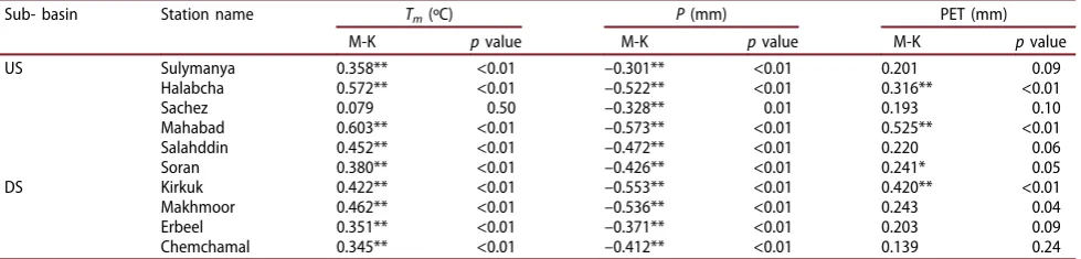
Table 2.Statistical properties of the meteorological variables after applying a nonparametric test for decadal change. US: upstream; DS: downstream. M-K: Mann-Kendall nonparametric test; Tm: mean air temperature; P: precipitation; PET: potential

evapotranspiration.

Sub- basin Station name _Tm(ºC) P(mm) PET (mm)

M-K pvalue M-K pvalue M-K pvalue US Sulymanya 0.358** <0.01 –0.301** <0.01 0.201 0.09

Halabcha 0.572** <0.01 –0.522** <0.01 0.316** <0.01 Sachez 0.079 0.50 –0.328** 0.01 0.193 0.10 Mahabad 0.603** <0.01 –0.573** <0.01 0.525** <0.01 Salahddin 0.452** <0.01 –0.472** <0.01 0.220 0.06 Soran 0.380** <0.01 –0.426** <0.01 0.241* 0.05 DS Kirkuk 0.422** <0.01 –0.553** <0.01 0.420** <0.01 Makhmoor 0.462** <0.01 –0.536** <0.01 0.243 0.04 Erbeel 0.351** <0.01 –0.371** <0.01 0.203 0.09 Chemchamal 0.345** <0.01 –0.412** <0.01 0.139 0.24 Negative (_–) and positive values indicate decreasing and increasing trends, respectively.

Downloads?Items=Software), applying the methodology developed by Mohammed and Scholz (2016).

The RS MINERVE 2.5 (2016) free software was applied for the simulation of free surface runoff flow formation and propagation (Foehnet al.2016), and used to run the HBV (Hydrologiska Byråns Vattenbalansavdelning) rain-fall–runoff model (https://www.crealp.ch/down/rsm/ install2/archives.html). To detect trends in the long-term hydro-climatic data, the distribution-free Mann-Kendall (M-K) method was applied (Tabari and Talaee 2011, Robaa and AL-Barazanji2013). This powerful technique does not assume a specific data distribution (Mohammed and Scholz2017a).Table 2presents the M-K test results for the key meteorological variables.

2.5 Hydrological model and climatic scenario

Rainfall–runoff models have been used widely to obtain streamflow data since such data are not easily obtainable. These models contain a series of equations that attempt to simulate the variety of the interrelated procedures that participate in hydrological processes. The hydrological models are usually categorized based on many criteria, such as process description, solution mechanism and scale. Many types of rainfall–runoff models have been used in the literature, such as lumped, distributed, con-tinuous-time and event-based models, as well as concep-tual and black-box models (Kaleris and Langousis2017). Based on a set of weather data, this research study applied the HBV rainfall–runoff model to simulate the basin runoff (Mohammedet al. 2018). The HBV is an illustration of a semi-distributed conceptual model esti-mating daily discharge based on daily precipitation and temperature, and monthly estimates of potential evapora-tion as input data. For runoff simulaevapora-tion, the model was initially calibrated and subsequently validated for normal climate. The performance of the HBV model was evalu-ated by using the following statistical criteria:

RMSE¼

ffiffiffiffiffiffiffiffiffiffiffiffiffiffiffiffiffiffiffiffiffiffiffiffiffiffiffiffiffiffiffiffiffiffiffiffiffiffiffiffiffiffiffiffiffiffi

1

n

Xn

i¼1

R_{obsð Þi} R_{simð Þi}

2

s

(9)

IoA¼1

Pn

i¼1 RobsðiÞRsimðiÞ

2

Pn

i¼1

R_obsðiÞRobs

_þR_simðiÞRobs

2 (10)

r¼

ffiffiffiffiffiffiffiffiffiffiffiffiffiffiffiffiffiffiffiffiffiffiffiffiffiffiffiffiffiffiffiffiffiffiffiffiffiffiffiffiffiffiffiffiffiffiffiffiffiffiffiffiffiffiffiffiffiffiffiffiffiffiffiffiffiffiffiffiffiffiffiffiffiffiffiffiffiffiffiffiffiffiffiffiffiffiffiffiffiffiffiffiffiffiffiffiffi_P

n

i¼1 Robsð Þi Robs

Rsimð Þi Rsim

Pn

i¼1 Robsð Þi Robs

0:5 Pn

i¼1 Rsimð Þi Rsim

0:5

v u u t

(11)

MAE¼1

n

Xn

i¼1

Robsð Þi Rsimð Þi

(12)

where RMSE is the root mean square error (–), IoA is the index of agreement (–), ris the correlation coeffi-cient (–), MAE is the mean absolute error,Robs(i)is the

measured streamflow (mm/month) at time stepi,Rsim (i)is the predicted streamflow (mm/month) at time step

i, Robsis the average amount of the recorded values

(mm/month) andn is the number of data point(s). For the climate change prediction, the delta perturba-tion scenario was applied (Tigkas et al. 2012, Al-Faraj

et al. 2014, Mohammed and Scholz 2017b, 2018). By using this scenario, the historical climatic variables (mean air temperature and/or precipitation) are per-turbed incrementally (and rationally) through arbitrary amounts, as shown in Equation (13), with steps of 2% within the range 0 to−40% forPand 0 to +30% for PET. These scenarios comprise all potential basinwide climate change predictions (336 scenarios).

AMVt¼OMVtRAOMVt (13)

where AMVtis the anticipated meteorological variable

(mm) at a specific time step t, OMVtis the observed

meteorological variable (mm) at time steptand RA is the added or subtracted ratio (%).

To simulate different climate change scenarios, we used the hydrological years 1988–2000, which are characterized by a mean of RDIstnear to zero. Even though the delta

perturbation scenario does not address changes in the probability distribution of weather properties and season-ality of, for example, streamflow in the future, it is still a productive technique for identifying tipping points when a reservoir is anticipated to fail catastrophically in supplying sufficient water (Mohammed and Scholz2017b). The delta perturbation scenarios often represent a realistic set of variations that are physically reasonable. Recently, numer-ous researchers have adopted this scenario (e.g. Tigkas

et al. 2012, Al-Faraj and Scholz 2014, Reis et al. 2016, Soundharajanet al.2016, Mohammed and Scholz2017b).

3 Findings and discussion

3.1 Meteorological parameter trends

To identify the decadal trend of the main meteorological variables, a distribution-free test was conducted.Table 2

shows the analysis for 10 meteorological stations dis-tributed between the upstream and downstream sub-basins for the time horizon between 1979 and 2013. The analysis shows that there is a positive tendency in yearly mean temperature (Tm) at approximately 90%

(p < 0.01) of the locations. The significant warming trends in yearly Tm changed from 0.37 to 1.91°C per

UNESCO 2014, Mulder et al. 2015, Mohammed et al.

2017b). A declining trend in precipitation with an aver-age degrease of about 162 mm per decade was observed (Fig. 3(a)). The basin annual and maximum precipita-tion are approximately 720 and 1222 mm, respectively, whereas the equivalent lowest 250 mm was allocated to the period 2007–2008. Statistical analysis of the meteor-ological data revealed that the climate of the study area has been getting warmer and drier due to climate change over the past 35 years.

Furthermore, the average yearly precipitation altered spatially from 56 mm at Kirkuk station, which is located in the lower sub-basin, to 1369 mm at Sulymaniya station, located in the upper sub-basin. This shows that the upstream sub-basin, which is considered high com-pared to the downstream sub-basin, had greater preci-pitation values than the downstream one.

The analysis also showed that long-term PET has risen significantly (p < 0.01), by approximately 77%, with a decadal growth that extended to a maximum of about 36 mm (Table 2). Both variations have contributed signifi-cantly (p< 0.01) to the decrease in river flow and indicate that, during the past 35 years, climate change has affected the meteorological characteristics of the LZRB consider-ably. Climate variation produced changes in precipitation, mean temperature and potential evapotranspiration, extending the gap between the basin water storage cap-ability and the equivalent water needs (Fig. 3(a) and (b)).

3.2 Baseflow index analysis

3.2.1 Spatio-temporal distribution

3.2.1.1 Upstream sub-basin. Based on the outcomes of Equation (7), a value of α = 0.982 yielded a BFI equivalent to the value resulting from the low-flow analysis. After considering this value in the baseflow separation technique, the following information was gained: firstly, over the hydrological period 1931–2013, the annual baseflow values varied from 0.448 × 109 m3 (2006) to 3.54 × 109 m3 (1968). The equivalent annual baseflow varied from nearly 37 m3to almost 293 m3. However, the long-term baseflow value and the equivalent standard deviation (SD) were 1.43 × 109 and 0.60 × 109 m3, respectively. Accordingly, the long-term average annual value of baseflow and the associated SD were predicted to be around 118 and ~50 mm, respectively. The results show that the storage of the Dokan sub-basin aquifer decreased by about 87%, which indicates that during the past 35 years climate change has negatively affected the availability of water within the basin.

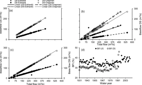
Figure 4((a)–(c)) and Equations (14), (20) and (26) (Table 3) show a strong correlation between the separated

baseflow and the total flow. Furthermore, Figure 4(d) shows that the annual temporal values of the BFI fluctu-ated from 0.26 (1958) to 0.42 (1997) and the long-term BFI and the equivalent SD were 0.35 and 0.027, respectively. These outcomes show that around 70% of the yearly BFI values were located within the mean ± SD ranges.

Based on Equation (8), the results show that a value ofα= 0.925 yields a BFI equivalent to the value gained from the FDC. Therefore, the annual values of baseflow changed from 0.84 × 109 m3 (2006) to 7.26 × 109 m3 (1968). The equivalent annual baseflow varied from ~69 mm to ~600 mm. The long-term average annual value of baseflow and the equivalent SD were 2.86 × 109 and 1.23 × 109m3, respectively. The long-term average yearly value of baseflow and the corre-sponding SD were 237 and ~102 mm, respectively. The results of Equation (8) also show that the storage of the Dokan sub-basin aquifer decreased by about 88%, which confirms the results obtained by applying Equation (7) and indicates that, during the past 35 years, climate change has negatively affected the availability of water within the basin.

Figure 4shows the separated baseflow linked with the total flow. The developed linear models (Equations (15), (21) and (27); Table 3) also show a strong correlation. The temporal variation of annual

BFI ranged from 0.51 (1968) to 0.54 (1972). The average long-term BFI value and the matching SD were 0.53 and 0.01, respectively. Accordingly, roughly 61% of the BFI yearly values were expected to be within the mean ± SD ranges. Furthermore, the results demonstrated a good relationship between

Equations (7) and (8), as shown in Table 3

(Equations (16), (22) and (28)).

The BFI, which is the ratio Q90/Q50, represents volumes

of water that the river might have obtained from ground-water flow or other delayed shallow subsurface sources in the studied periods. A high BFI value shows the ability of

Figure 4.Linear regression models for the relationships between the separated baseflow using Eckhardt and Chapman methods and the total runoff at upstream (US) and downstream (DS) sub-basins for (a) pre-damming, (b) post-damming, and (c) integrated time periods; and (d) annual baseflow index (BFI) variability as a function of time for the US and the DS sub-basins, estimated by the Eckhardt recursive digital filtering algorithms coupled with the flow–duration curve (FDC).

Table 3.Linear regression models developed for the upstream and downstream sub-basins and the three considered time periods using the Eckhardt algorithm linked to the flow duration curve and the Chapman digital algorithm. BF: baseflow; TF: total flow. BFE: Eckhardt BF; BFC: Chapman BF.

Time period Sub-basin Algorithm Equation formulation R2 _{Equation no.}

Pre-damming Upstream Eckhardt BF = 0.24TF + 1.3 0.99 (14) Chapman BF = 0.48TF + 2.7 0.92 (15) Eckhardt-Chapman BFE= 1.95BFC+ 0.65 0.91 (16)

Downstream Eckhardt BF = 0.25TF + 0.1 0.99 (17) Chapman BF = 0.51TF−3.6 0.97 (18) Eckhardt-Chapman BFE= 2.10BFC−3.73 0.97 (19)

Post-damming Upstream Eckhardt BF = 0.23TF + 5.0 0.80 (20) Chapman BF = 0.48TF + 1.3 0.99 (21) Eckhardt-Chapman BFE= 1.70BFC+ 11.1 0.80 (22)

Downstream Eckhardt BF = 0.12TF + 0.2 0.99 (23) Chapman BF = 0.52TF−5.2 0.99 (24) Eckhardt-Chapman BFE= 4.20BFC−6.2 0.99 (25)

Integrated Upstream Eckhardt BF = 0.24TF + 1.8 0.97 (26) Chapman BF = 0.52TF−5.2 0.99 (27) Eckhardt-Chapman BFE= 2.10BFC−5.2 0.99 (28)

the basin to recharge the stream during a prolonged dry season. The BFI is associated with many river basin char-acteristics, such as soil type and geology, topography, vegetation and weather. Analysis of the results indicates that there is a moderate variation in the BFI values at the upstream sub-basin, which can be attributed to the increase in groundwater influence on the total flow of the river. Therefore, more consideration should be given to evaluating the aquifer characteristics and comprehending the aspects that might cause such alterations for improving management of subsurface resources within the basin.

3.2.1.2 Downstream sub-basin. The results from Equation (7) show that a value ofα= 0.925 yields a BFI equating to that obtained from the FDC. For the period 1931–1993, the annual baseflow magnitude changed between 0.01 × 109m3(1993) and 4.20 × 109m3(1968). The long-term average yearly baseflow value and the equivalent SD were 1.60 × 109and 0.76 × 109m3, respec-tively.Figure 4shows the relationships between the entire flow and the separated baseflow. The estimated linear model represented by Equations (17), (23) and (29) (Table 3) shows a good correlation. However,Figure 4(d) shows that the annual temporal values of BFI varied from 0.26 (1968) to 0.82 (1992), with 0.30 and 0.12 long-term BFI and SD, respectively. These outcomes indicate that nearly 94% of the yearly BFI values are within the mean ± SD ranges.

Based on Equation (8), a value ofα= 0.925 creates a BFI that is equivalent to the value estimated by the FDC. During the period 1931–1993, the annual baseflow values varied from 0.01 × 109m3(1993) to 8.42 × 109m3(1968). The long-term average yearly baseflow value and SD were 3.08 × 109and 1.61 × 109m3, respectively. The values of BFI varied between 0.21 (1989) and 0.82 (1992), while the BFI long-term value was 0.51 ± 0.11. Around 94% of the baseflow index annual values are within the mean ± SD ranges range and the developed Equations (18), (24) and (30) (Table 3) show a robust coefficient of determination (R2). The results also demonstrate a strong relationship between Equations (7) and (8), as shown in Table 3

(Equations (19), (25) and (31)).

The results of Equations (7) and (8) are identical at the downstream sub-basin and show that there was a reduction in the storage of the sub-basin aquifer by about 100%; they also indicate that, during the past 35 years, climate change has negatively affected the availability of water within the basin. Furthermore, the temporal analysis of the BFI indicates that, during the hydrological year 1968, the contribution of the ground-water to the LZRB total hydrograph was larger (about 74%) than that during the hydrological year 1989, which

may be attributed to the reduction of the basin water storage availability as a result of climate change.

The spatial analysis of the BFI shows that the filter parameter values of 0.982 and 0.925, which were obtained from Equations (7) and (8), respectively, are not the same for the upper and lower sub-basins, and this shows that the aquifers of the two sub-basins have different features. Accordingly, to improve the water resources manage-ment of the basin, more attention should be given to assessing the characteristics of the aquifer and compre-hending the aspects that might cause such differences.

3.2.2 Human-induced impact

To explore the potential impact of human activities (i.e. river damming) on the subsurface water contribution to the total streamflow, this study considered three time periods representing pre-damming, post-damming and an integrated time period. At the upstream sub-basin, the pre-damming period covers the hydrological years 1931–1965, the post-damming period covers the hydro-logical years 1966–2013, and the integrated period covers the hydrological years 1931–2013. The corresponding periods at the downstream sub-basin are 1931–1965, 1966–1993 and 1931–1993, respectively.

At the upstream sub-basin (Dokan), the Q90and Q50

values for the three considered periods were 35 and 101, 31 and 100, and 33 and 100 m3/s, respectively. Thus the Q90/Q50ratios were 35, 31 and 33%, respectively,

repre-senting the water capacities that the stream would obtain from groundwater recharge and/or other delayed low groundwater resources during the considered time periods. At the downstream sub-basin (Altun Kupri-Guma Zerdela), the corresponding Q90 and Q50 values

were 40 and 132, 17 and 127, and 31 and 129 m3/s, respectively, with Q90/Q50ratios of 30, 14 and 24%.

The results show that the BFI values for the pre-dam-ming periods were considerably larger than those for the post-damming and integrated periods, and this can be attributed to the decrease in the subsurface water con-tribution to the LZRB flow due to water being stored by the Dokan Reservoir throughout dry months. This, in turn, decreases the BFI. Consequently, and for the pur-poses of the development of groundwater flow manage-ment, more attention should be given to the evaluation of the groundwater aquifer properties and to understanding the features potentially causing these variations.

during the same period varied from 1.38 × 109m3(1958) to 5.71 × 109m3(1953) and the equivalent annual base-flow was between 65 and 266 mm. The long-term annual mean BF was 2.91 ± 1.05 × 109m3.

For the post-damming period, the annual baseflow values obtained from Equation (7) varied between 0.437 × 109m3(2006) and 3.647 × 109m3(1968). The equivalent annual baseflow changed from about 21 to 170 mm. The long-term annual mean baseflow volume was 1.45 ± 0.70 × 109m3. Using Equation (8), the annual baseflow values varied from 0.871 × 109 m3 (2006) to 7.077 × 109m3(1968) and the equivalent annual baseflow changed from approximately 40 to 330 mm. The long-term annual mean baseflow was 2.88 ± 1.31 × 109 m3. These findings show that, due to the impact of climate change over the past 35 years, the basin aquifer storage decreased by about 77 and 88% for pre-regulated and post-regulated time periods, respectively. This may directly affect the availability of water within the basin.

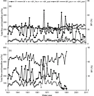
Furthermore, Figure 5 displays the variations in total flow, baseflow and BFI for the three periods in the two sub-basins, and shows that the derived base-flow values for the studied time periods display similar patterns. Variations were seen for the BFI in the

post-damming period, in particular, at the upstream sub-basin (Fig. 5(a)), which could be attributed to the water stored in the Dokan Reservoir during the dry season.

3.2.3 Impact of drought and climate change

To study the impact of climate change and drought phenomena on basin hydrology, it is important (as a first step) to investigate the impact of such changes on the hydro-climatic variables and the baseflow index. The dry and wet years are determined by the minimum and the maximum flows, respectively. Yoo (2006) suggested that when the average yearly precipitation of the basin is greater than the average precipitation (Pav) + 0.75SD,

then the hydrological year is defined as wet. However, when precipitation is no more than the characterizedPav

−0.75SD, the year is considered as dry. Therefore, years with annual precipitation values within this range can be regarded as normal hydrological years, i.e.Pav−0.75SD≤

P≤Pav+ 0.75SD (Yanget al.2008).

Figure 6shows wet- and dry-year thresholds coupled with precipitation and BFI. A significant (p< 0.01) rise in the basin average precipitation,Pav, of nearly 44% was seen

for the year 1987. A noteworthy change in the flow of about 118% resulted in an increase in the amount of precipitation,

which in turn reduced the groundwater involvement in the total flow. In contrast, the periods 1998–2001 and 2006–2008 are linked to a steep drop inPavof

approxi-mately 40 and 60%, respectively. A decline of about 66, 77 and 79% in river flow (the equivalent annual average flow of 0.35 × 109, 0.31 × 109 and 0.34 × 109 m3) for the hydrological years 1998/99, 1999/00 and 2000/01, respec-tively, resulted from the reduction in basin average preci-pitation, which caused an increase in the groundwater contribution (represented by the BFI). Nevertheless, 52, 80 and 83% streamflow decreases (equivalent to annual mean flow volumes of 0.76 × 109, 0.29 × 109 and 0.31 × 109 m3) were observed during the hydrological years 2006/07, 2007/08 and 2008/09, respectively. Additionally, the period 1991‒2013 experienced a steep drop in flow, during which the flow change ranged between 75 and 86% (equivalent to 0.31 × 109and 1.24 × 109m3), indicating the absolute minimum and maximum yearly average storage capacities; simultaneously, the baseflow increased from approximately 31 to nearly 35%.

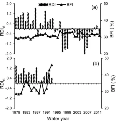
Figure 7presents RDIstvalues estimated for the studied

sub-basins, showing that a non-symmetric annual pattern of droughts and wet periods was detected, particularly in the upper sub-basin. These results indicate that the studied area suffered from a severe drought during the last few decades and the severity of drought increased, while the

number of months with long durations of precipitation shortages and potential evapotranspiration growth increased. Droughts were identified on a regular basis at the upstream sub-basin for the hydrological years 1998/99, 1999/2000, 2000/01, 2007/08 and 2008/09 (Fig. 11(a)). The corresponding mean RDIstvalues were−1.84,−1.67,−1.45,

−2.91 and−1.53. These findings, which complement sev-eral earlier studies (Fadhil2011, UNESCO2014), indicate that climate change has increased the severity of droughts within the studied climatic zone. At the upstream sub-basin (Fig. 7(a)) the baseflow index increased from approximately 30 to 35%, while at the downstream sub-basin (Fig. 7(b)) no drought episodes were recorded.

3.2.4 Seasonal analysis

Furthermore, results of the seasonal BFI variability at the upstream sub-basin (Fig. 8(a)) show that this sub-basin is likely to recharge LZRB with groundwater. This contribution started to rise significantly (p< 0.05) from April, reaching an absolute maximum by the end of June. Then, this level of recharge continued without change until the middle of August, followed by a mar-ginal drop in September. In general, the BFI entries showed high variations over the dry period.

Figure 6.Long-term baseflow index (BFI) with both wet- and dry-year thresholds coupled with long-term average precipita-tion for the period 1979–2013 for (a) Dokan and (b) Altun Kupri-Goma Zerdela stations. Note: For Altun Kupri station, there are no data available for the period 1995–2013.

Figure 8(b) reveals that the long-term BFI at the down-stream sub-basin is nearly double that of the updown-stream sub-basin for the months October–April, whereas they are close to each other for the remaining period. This varia-bility in BFI may result from the difference in the studied time periods, since the period horizon for the Dokan sub-basin spanned from 1931 to 2013 (82 years), whereas that for the Altun Kupri-Goma Zerdela sub-basin ranged from 1931 to 1993 (62 years). Despite the fact that the catch-ment area of the Dokan sub-basin (12 096 km2) is larger than that of the Altun Kupri-Goma Zerdela (8509 km2), the former is characterized by both a higher precipitation rate and elevation (Table 4). This would increase the contribution of runoff and the interflow to the total flow of the Dokan sub-basin, which in turn decreases the con-tribution of the baseflow to the LZRB discharge. The

research findings specify that, over the last few years, climate variability and drought events harmfully affected the water resources availability of LZRB.

Figure 9 reveals the anticipated variations of RDIst

associated with the potential impact of future reduction in the precipitation under the collective effect of potential evapotranspiration increase. Figure 9indicates that the severity of drought would increase as a result of climate change.

Furthermore, considering the climate change impacts on the separated baseflow as well as the inflow to the Dokan Reservoir, Figure 10 (baseflow) and Figure 11

(inflow) show examples of the sensitivity analysis of these hydrological characteristics under the collective impacts of climate change.

The HBV model has been used to simulate the reser-voir inflow, which was firstly calibrated and validated based on the normal climatic conditions. During the model calibration, the statistical performance results of RMSE, index of agreement (IoA), correlation coefficient (r) and mean average error (MAE), were 0.73, 0.99, 0.93 and 0.65, respectively, whereas the values for the valida-tion period were 0.68, 0.99, 0.84 and 0.60 (refer also to

Figure 8.Seasonal variations of baseflow index (BFI) estimated by the Eckhardt filtering algorithm coupled with the flow–duration curve for the three studied time periods at (a) Dokan and (b) Altun Kupri-Goma Zerdela. Note: For Altun Kupri station, there are no data available for the period 1995–2013.

Table 4.Station locations with corresponding average precipitation and the sub-area sizes. US: upstream; DS: downstream; Lat.: latitude; Long.: longitude; Elev.: elevation; Pav: average precipitation; and PETav: average potential evapotranspiration.

Sub-basin Station Lat. (°) Long. (°) Elev. (m a.s.l.) Sub-area (km2_{) P}

av(mm) PETav(mm)

US Sulymaniya 35.53 45.45 885 4479.57 772 1989 Halabcha 35.44 45.94 651 735.60 585 980 Sachez 36.25 46.26 1536 1182.79 462 1550 Mohabad 36.75 45.70 1356 2593.31 886 920 Salahddin 36.38 44.20 1088 1641.07 652 2058 Soran 36.87 44.63 1132 1463.30 813 1433 DS Kirkuk 35.47 44.40 319 1693.76 342 897

Makhmoor 35.75 43.60 306 3008.41 361 934 Erbil 36.15 44.00 1088 979.76 575 935 Chemchamal 35.52 44.83 701 2827.46 738 2075

Mohammed and Scholz2017b). The findings emphasize that the model can confidently be used for more research, such as running the delta perturbation scenarios and calculating the relative change (%) of mean yearly flow relative to the natural climate conditions.

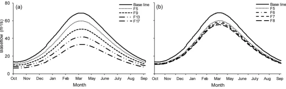
Figures 10(a)and11(a) show that the baseflow and reservoir inflow are sensitive to seasonal variations in precipitation. However, they can be considered less sensitive to the variations of potential evapotranspira-tion (Fig. 10(b) and 11(b)). Additionally, Figures 10

and 11 demonstrate how climate change could cause marked drops in the separated baseflow and reservoir inflow. Compared to the baseline and the observed inflow values, the peaks of the anticipated values of these variables would decrease and there would be a noticeable alteration in their magnitude, which could lead to a dramatic impact on the water resources avail-ability of the basin.

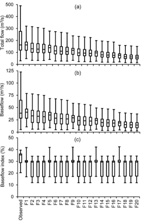
Figure 12shows that there would be a wide variability in the simulated inflow, baseflow and BFI values. For example, the simulated values of inflow, baseflow and

BFI based on the Future 6 scenario (F6) (10%

precipita-tion reducprecipita-tion linked with 10% potential evapotran-spiration increase) could be as low as 36, 34 and 22%, respectively, which indicates the severity of climate change in the study area. The climate change impact on the runoff estimations generally follows the impact on both baseflow and BFI. The coefficient of variation (Cv) for the simulated inflow, separated baseflow and BFI is as high as 0.45, 0.51 and 0.31, respectively. This coefficient can be considered as an indication of the variability or uncertainty of these values.

4 Conclusions and recommendations

A generic methodology was applied to evaluate the impact of climate change, drought phenomena and anthropogenic activities on the baseflow contribution to the total flow of an arid basin. The results indicate that there was a similar pattern in the annual temporal variations of the separated baseflow for the upstream and downstream parts of the basin. Very good correlations were noticed between the

Figure 10.Sensitivity analysis of the separated baseflow with respect to the impact of (a) precipitation (P) reduction and (b) potential evapotranspiration (PET) increase. Future scenarios: F5 (10% reduction in P linked with 0% increase in PET); F6, F7 and F8 (10% reduction inPlinked with 10, 20 and 30% increase in PET, respectively); and F9(20% reduction inPlinked with 0% increase in PET).

separated baseflow and the total flow at both locations, as well as between the two considered algorithms. The aver-age yearly baseflow index increased from 0.14 to 0.38 for the upstream and downstream sub-basins, respectively, which indicates that 14–38% of the long-standing flow of the basin can be sustained by groundwater flow. There were relatively large differences in the baseflow contribu-tions between the upstream and downstream sub-basins, which can be attributed to the variations in the studied periods and the drainage area of each sub-basin, as well as the existence of aquifers with greater releases in the down-stream location compared to the updown-stream one.

Alteration of the hydrological environment can be con-sidered as one of the significant potential impacts of the projected climate change in the reservoir area. Based on the outputs of the HBV model, a serious reduction in the Dokan Reservoir inflow is recommended due to the

reduced precipitation and the rise in potential evapotran-spiration. For example, a decrease in streamflow of approximately 21% is likely to result in 10% precipitation decrease and 30% potential evapotranspiration increase. The peak inflow value will decrease and there will be a clear shift in the corresponding magnitude, which would lead to a significant impact on the availability of water resources within the basin.

The suggested approach is useful, simple and sup-ports the preparation for future basin management, particularly when challenging hydrological models can-not be applied appropriately because of a deficiency in the observed data. This method bridges the gap in the understanding of decision makers with respect to the influence of climate variability, drought phenomena and human activities on the baseflow contribution to streamflow under arid climatic conditions.

Further research is recommended to evaluate the aqui-fer behaviour and the corresponding data variability. A detailed exploration of the baseflow contribution to the total flow is important, because of water resources shortages and corresponding conflicts among different stakeholders and countries. Furthermore, the study should be repeated for different climatic regions to assess climate change in addition to the impact of both drought phenomena and river regulation on groundwater contri-butions to runoff.

Disclosure statement

No potential conflict of interest was reported by the authors.

Funding

The researchers received funding from the Government of Iraq via Babylon University for the PhD studies by the lead author.

References

Al-Faraj, F. and Scholz, M.,2014. Incorporation of the flow duration curve method within digital filtering algorithms to estimate the baseflow contribution to total runoff. Water Resources Management, 28 (15), 5477–5489. doi:10.1007/s11269-014-0816-7

Al-Faraj, F., Scholz, M., and Tigkas, D.,2014. Sensitivity of surface runoff to drought and climate change: application for Shared River Basins.Water, 6, 3033–3048. doi:10.3390/w6103033 Allen, R.G., et al., 1998. Crop evapotranspiration: guidelines

for computing crop water requirements. Rome, Italy: Food and Agriculture Organization of the United Nations, FAO Irrigation and Drainage Paper 56.

Arnold, J.G. and Allen, P.M.,1999. Validation of automated methods for estimating baseflow and groundwater

recharge from stream flow records. Journal of the

American Water Resources Association, 35 (2), 411–424. doi:10.1111/j.1752-1688.1999.tb03599.x

Brodie, R.S. and Hostetler, S., 2005. A review of techni-ques for analyzing base-flow from stream hydrographs. Proceedings of the NZHSIAH-NZSSS 2005 Conference,

28 November–2 December 2005, Auckland, New

Zealand. Available from: http://data.daff.gov.au/data/

warehouse/brsShop/data/iah05_dry-weather_final.pdf.

[Accessed 11 June 2018].

Chapman, T.,1999. A comparison of algorithms for

stream-flow recession and basestream-flow separation. Hydrological

Processes, 13 (5), 701–714. doi:10.1002/(SICI)1099-1085 (19990415)13:5<701::AID-HYP774>3.0.CO;2-2

Eckhardt, K.,2005. How to construct recursive digital filters for baseflow separation. Hydrological Processes, 19, 507– 515. doi:10.1002/hyp.5675

Fadhil, M.A.,2011. Drought mapping using Geoinformation technology for some sites in the Iraqi Kurdistan region. International Journal of Digital Earth, 4 (3), 239–257. doi:10.1080/17538947.2010.489971

Fan, Y., et al., 2013. Variation of baseflows in the

head-streams of the Tarim River Basin during 1960–2007.

Journal of Hydrology, 487, 98–108. doi:10.1016/j. jhydrol.2013.02.037

FAO (Food and Agriculture Organization of the UN).2012. Adaptation to climate change in semi-arid environments. Experience and lessons from mozambique. Environment and natural resources management series. Rome, Italy: Food and Agriculture Organization of the United Nations, 1–83, Retrieved from, http://www.fao.org/doc rep/015/i2581e/i2581e00.pdf

Foehn, A., et al., 2016. RS MINERVE –user’s manual v2.6. Switzerland: RS MINERVE Group.

GADM (Global Administrative Areas Database), 2012.

Boundaries without limits[online]. Available fromhttp:// www.gadm.org. [Accessed 11 June 2018].

GLCF (Global and Land Cover Facility),2015.Earth science data interface [online]. Available from: http://www.land cover.org/data/srtm/. [Accessed 11 June 2018].

Gordon, N.C.,et al.,2004.Stream hydrology: an introduction for ecologists. 2nd ed. Chichester: John Wiley and Sons. He, S.,et al., 2016. Baseflow separation based on a

meteor-ology-corrected nonlinear reservoir algorithm in a typical rainy agricultural watershed. Journal of Hydrology, 535, 418–428. doi:10.1016/j.jhydrol.2016.02.010

HydroOffice, 2015. Download [online]. Available from:

https://hydrooffice.org/Downloads?Items=Software. [Accessed 11 June 2018].

Information Technology Services (ITS), 2016. IBM SPSS

statistics 23 Part 3: regression analysis. Winter 2016, Version 1.

Kaleris, V. and Langousis, A., 2017. Comparison of two

rainfall-runoff models: effects of conceptualization,

model calibration and parameter variability.Hydrological Sciences Journal, 62 (5), 729–748. doi:10.1080/ 02626667.2016.1250899

Lim, K.J.,et al.,2005. Automated web GIS based hydrograph

analysis tool, WHAT. Journal of the American Water

Resources Association, 41 (6), 1407–1416. doi:10.1111/ j.1752-1688.2005.tb03808.x

Linsley, R.K., Kohler, M.A., and Paulhus, J.L.H., 1988. Hydrology for engineers. London: McGraw-Hill.

Lott, D.A. and Stewart, M.T.,2016. Baseflow separation: A com-parison of analytical and mass balance methods.Journal of Hydrology, 535, 525–533. doi:10.1016/j.jhydrol.2016.01.063 Lu, S.,et al.,2015. Quantifying impacts of climate variability

and human activities on the hydrological system of the

haihe river basin, China. Hydrology and Earth System

Sciences, 73, 1491–1503. doi:10.1007/s12665-014-3499-8 Mei, Y. and Anagnostou, E.N.,2015. A hydrograph

separa-tion method based on informasepara-tion from rainfall and

run-off records. Journal of Hydrology, 523, 636–649.

doi:10.1016/j.jhydrol.2015.01.083

Miller, M.P., et al., 2016. The importance of baseflow in sustaining surface water flow in the upper colorado river

basin. Water Resources Research, 52, 3547–3562.

doi:10.1002/2015WR017963

Mohammed, R. and Scholz, M., 2016. Impact of climate

variability and streamflow alteration on groundwater con-tribution to the baseflow of the Lower Zab River (Iran and Iraq). Environmental Earth Sciences, 75 (1392), 1–11. doi:10.1007/s12665-016-6205-1

Mohammed, R. and Scholz, M., 2017a. The reconnaissance

drought index: a method for detecting regional arid cli-matic variability and potential drought risk. Journal of Arid Environment, 144, 181–191. doi:10.1016/j. jaridenv.2017.03.014

Mohammed, R. and Scholz, M., 2017b. Adaptation strategy to mitigate the impact of climate change on water resources in arid and semi-arid regions: a case study. Water Resources Management, 31 (11), 3557–3573. doi:10.1007/s11269-017-1685-7

Mohammed, R. and Scholz, M.,2017c. Impact of evapotran-spiration formulations at various elevations on the

recon-naissance drought index. Water Resources Management,

31, 531–538. doi:10.1007/s11269-016-1546-9

Mohammed, R. and Scholz, M.,2018. Climate change and

anthropogenic intervention impact on the hydrologic anomalies in a semi-arid area: lower Zab River Basin,

Iraq. Environmental Earth Sciences, 77 (10), 357.

doi:10.1007/s12665-018-7537-9

Mohammed, R.,et al., 2018. Assessment of models predict-ing anthropogenic interventions and climate variability on

surface runoff of the Lower Zab River. Stochastic

Environmental Research and Risk Assessment, 32 (1), 223–240. doi:10.1007/s00477-016-1375-7

Mohammed, R., Scholz, M., and Zounemat-Kermani, M., 2017b. Temporal hydrologic alterations coupled with cli-mate variability and drought for transboundary river

basins. Water Resources Management, 31, 1489–1502.

doi:10.1007/s11269-017-1590-0

Mulder, G.,et al., 2015. Identifying water mass depletion in

northern Iraq observed by GRACE. Hydrology and Earth

System Sciences, 19, 1487–1500. doi: 10.5194/hess-19-1487-2015

Nathan, R.J. and McMahon, T.A.,1990. Evaluation of auto-mated techniques for baseflow and recession analysis. Water Resources Research, 26, 1465–1473. doi:10.1029/ WR026i007p01465

The Nature Conservancy,2009. Indicators of hydrologic altera-tion version 7.1 user’s manual. The Nature Conservancy, June, 76.

baseflow from a physically based, surface water-ground-water flow model.Journal of Hydrology, 458–459, 28–39. doi:10.1016/j.jhydrol.2012.06.029

Piggott, A.R., Moin, S., and Southam, C., 2005. A revised approach to the UKIH method for the calculation of base-flow/Une approche améliorée de la méthode de l’UKIH pour le calcul de l’écoulement de base. Hydrological Sciences Journal, 50, 911–920. doi:10.1623/hysj.2005.50.5.911 Price, K.,2011. Effects of watershed topography, soils, land

use, and climate on baseflow hydrology in humid regions: a review.Progress in Physical Geography, 35 (4), 465–492.

doi:10.1177/0309133311402714

Reis, J.,et al.,2016. Evaluating the impact and uncertainty of reservoir operation for malaria control as the climate

changes in Ethiopia. Climatic Change, 136, 601–614.

doi:10.1007/s10584-016-1639-8

Robaa, S.M. and AL-Barazanji, Z.J., 2013. Trends of annual

mean surface air temperature over Iraq. Nature and

Science, 11 (12), 138–145.

RS MINERVE 2.5 software, 2016. Download [online].

Available from: https://www.crealp.ch/down/rsm/install2/ archives.html. [Accessed 11 June 2018].

Rumsey, C.A.,et al., 2015. Regional scale estimates of base-flow and factors influencing basebase-flow in the upper color-ado river basin. Journal of Hydrology: Regional Studies, 4 (2015), 91–107. doi:10.1016/j.ejrh.2015.04.008

Smakhtin, V.U.,2001. Low flow hydrology: a review.Journal of Hydrology, 240 (3–4), 147–186. doi:10.1016/S0022-1694(00) 00340-1

Soundharajan, B.S., Adeloye, A.J., and Remesan, R., 2016. Evaluating the variability in surface water reservoir plan-ning characteristics during climate change impacts assess-ment. Journal of Hydrology, 538, 625–639. doi:10.1016/j. jhydrol.2016.04.051

Stewart, M.K.,2015. Promising new baseflow separation and recession analysis methods applied to streamflow at

Glendhu Catchment, New Zealand.Hydrology and Earth

System Sciences, 19 (6), 2587–2603. doi: 10.5194/hess-19-2587–2015

Tabari, H. and Taalaee, P.H., 2011. Analysis of trend in temperature data in arid and semi-arid regions of Iran. ISSN: 0921-8181.Global and Planetary Change, 72, 1–10. doi:10.1016/j.gloplacha.2011.07.008

Tallaksen, L.M. and Van Lanen, H.A., 2004. Hydrological drought–processes and estimation methods for streamflow and groundwater. Developments in Water Sciences 48. Amsterdam: Elsevier.

Tigkas, D.,2008. Drought characterisation and monitoring in regions of Greece.European Water, 23, 29–39.

Tigkas, D., Vangelis, H., and Tsakiris, G.,2012. Drought and climatic change impact on streamflow in small watersheds. ISSN: 0048-9697. Science of the Total Environment, 440, 33–41. doi:10.1016/j.scitotenv.2012.08.035

Tsakiris, G. and Vangelis, H.,2005. Establishing a drought index incorporation evapotranspiration.European Water, 9, 3–11. UNESCO,2014. United nations educational, scientific and

cul-tural organization. Integrated drought risk management-DRM national framework for Iraq. An analysis report. Available from: http://unesdoc.unesco.org/images/0022/

002283/228343E.pdfUN-ESCWA and BGR (United Nations

Economic and Social Commission for Western Asia;

Bundesanstalt für Geowissenschaften und Rohstoffe,

Inventory of Shared Water Resources in Western Asia, Beirut. Vangelis, H., Tigkas, D., and Tsakiris, G.,2013. The effect of PET method on reconnaissance drought index (RDI) cal-culation. Journal of Arid Environment, 88, 130–140. doi:10.1016/j.jaridenv.2012.07.020

Wan, L.,et al.,2015. Decadal climate variability and vulner-ability of water resources in arid regions of Northwest

China. Environmental Earth Sciences, 73, 6539–6552.

doi:10.1007/s12665-014-3874-5

Welderufael, W. and Woyessa, Y.,2010. Stream flow analysis and comparison of methods for baseflow separation: case study of the modder river basin in central South Africa. European Water, 8 (2), 107–119.

WMO (World Meteorological Organization),2009. Manual

of low-flow estimation and prediction, operational hydrology report no. 50. Geneva, Switzerland: World Meteorological Organization, WMO Report no. 1029. Yang, T., et al., 2008. A spatial assessment of hydrologic

alteration caused by dam construction in the middle and lower yellow river, China.Hydrological Processes, 22 (18), 3829–3843. doi:10.1002/hyp.6993