Performance Comparison of Linear and Decision Feedback Equalizers in Flat and Frequency Selective Fading Channel

(1)

International Journal of Emerging Technology and Advanced Engineering

Website: www.ijetae.com (ISSN 2250-2459,ISO 9001:2008 Certified Journal, Volume 3, Issue 10, October 2013)

668

Performance Comparison of Linear and Decision Feedback

Equalizers in Flat and Frequency Selective Fading Channel

Pradyumna Ku. Mohapatra

1

, Siba Prasad Panigrahi

2

, Jibanananda Mishra

3 1,3

Asistant Professor, OEC, BPUT, Bhubaneswar, ODISHA 2_{Professor, CVRCE, BPUT, Bhubaneswar, ODISHA}

Abstract—In this paper we have studied channel models (flat fading and frequency selective fading channels) estimation, adaptive equalization, and demodulation. The technique involves the optimization of the overall impulse response of the transmit and receive filters and effectively reduces the channel to one which is flat fading. This example showed the relative performance of linear and decision feedback equalizers in both flat and frequency-selective fading channels. It showed how a one-tap equalizer is sufficient to compensate for a frequency-flat channel, but that a frequency-selective channel requires an equalizer with multiple taps. Finally, it showed that a decision feedback equalizer is superior to a linear equalizer in a frequency-selective channel. Computer simulation results show that this equalization method works for channels with small delay spreads

Keywords—Channel models, Equalization, Fading, Frequency-selective, MIMO(Multiple Input Multiple Output),

I. INTRODUCTION

A radio channel exploits an extremely random characteristic, which does not allow us to use the simple AWGN channel model mentioned above to analyze the channel capacity. Radio signals propagate by means of reflection, diffraction, and scattering, which result in three effects a radio signal experiences: attenuation, large-scale shadowing, and small-scale fading. It was proved that these three effects are independent of each other. Signal attenuation is mainly introduced by the location of a receiver (distance between the transmitter and the receiver), which can be predicted by a deterministic model. Large-scale shadowing of a signal is mainly caused by multiple reflections and/or diffractions of the signal while propagating, whose characteristics can be captured with a log-normal distribution model. Small scale fading of a signal is caused by multiple versions of a transmitted signal with different delay times such that it has both time and location varying property. One type of channels with the fading effect caused by the multi-path time delay spread is flat fading channels in which the period of the transmitted signal is larger than the multi-path delay spread.

(2)

International Journal of Emerging Technology and Advanced Engineering

669 II. MOBILE WIRELESS CHANNELS

In wireless communications the transmitted signals arrives at the receiver along a number of different paths refered to as multipath shown in figure 2.1Multipath propagation arises due to reflection refraction and scattering of the electromagnectic wave on object such as buildings, hills, trees etc.that lie on the vicinity of transmitter/receiver user mobility (relative motion between transmitter/receiver) and or carrier frequency offset Induce time varrience on the channel.Hence wireless channel may be characterized by linear time varrying and multi-path fading.Multipath results into spreading of the transmitted signal in time(so called inter-symbol –interference ISI)),while time-variation of the channel results in to

frequency-spreading(the so called Doppler’ s spread)[4,5]

Figure1:The user signal experiences multipath propagation The selection of the channel model is linked to the transmitted signal characteristics, mainly based on the relationship between the transmitted signal bandwidth W and the channel coherence bandwidth or equivalently between the duration of the transmitted symbol T and the channel coherence time . In the following we will give a brief description of the different fading types

II (A). Frequency Non-Selective Fading Channel:

Let denote the frequency-domain representation of the transmitted signal. The noiseless received signal

at the receive antenna can be written as

Suppose that the transmitted signal bandwidth W is much smaller than the coherence bandwidth of the channel i. e Then all the frequency components of the transmitted signal will experience the same attenuation and phase shift. This means that the channel frequency response is fixed over the transmitted signal bandwidth W.

Such a channel is called frequency non-selective or frequency flat fading. Hence, for frequency flat fading channels the input-output relationship is reduced to

Where represents the time-varying envelop and represents the time-varying phase of the channel impulse response. From (2.5), we see that the frequency flat fading channel can be viewed as a multiplicative channel

II(B) Frequency-Selective Fading Channel

In this subsection we will treat the case when the transmitted signal bandwidth is larger than the coherence bandwidth of the channel, i.e. when In this case the different frequency components of the transmitted signal will experience different gains and phase shifts. In such a case, the channel is called frequency-selective. Contrary to the frequency flat case where the channel consists of one tap, the frequency-selective channel consists of multiple-taps (resolvable multipath). The multipath components are resolvable if they are separated in delay by . can be viewed as the time resolution of the receiver. For frequency-selective fading, the channel maximum delay spread . is much greater than the time resolution of the receiver . and therefore, echoes of the transmitted signal arrive at the receiver causing inter symbol interference (ISI). The signal echoes arrive at the receiver along a number of different resolvable paths (resolvable by the receiver time resolution

hence, the impulse response of the time-varying frequency-selective fading channel (or ISI channel) can be written as

(3)

International Journal of Emerging Technology and Advanced Engineering

670 Where L is the number of resolvable multipath components. Since the channel maximum delay spread is τmax, and the time resolution of the systems is 1/W ,the number of multipath components L is obtained as

The resolvable path of the multipath fading channel is characterized by its time-varying amplitude and its time-varying phase and can be written as

Therefore, the frequency-selective fading channel may be modeled by a tapped delay line with L+1 uniformly spaced taps. The tap spacing between adjacent taps is 1/W, and each tap is characterized by a complex-valued time-varying gain , as shown in Figure 2.3 [2].The frequency-selective channel reduces to frequency flat if L = 0 or the channel maximum delay spread is much smaller than the time resolution of the

receiver, i.e

II(C): Fast Fading vs. Slow Fading

In our discussion so far we consider the coherence bandwidth of the channel and its impact on the channel frequency selectivity. In this subsection we will consider the channel’s coherence time Tc and its impact on the channel time selectivity. The channel time selectivity determines whether the channel is slowly or fast fading

Figure.3 Type Of Small Scale Fading[1]

In fast fading, the channel impulse response changes rapidly within the symbol period T. In other words, the channel’s coherence time is smaller than the symbol period.

The time coherence of the channel is directly related to the Doppler spread, the larger the Doppler spread the smaller the coherence time and the faster the channel changes within the symbol period of the transmitted signal. Therefore, the transmitted signal is said to experience fast fading if In slow fading, the channel impulse response changes at a rate much slower than the symbol period of the transmitted signal. In this case the channel may be assumed to be static (invariant) over several symbol periods. Hence, the transmitted signal is said to experience slow fading if

(a) Time-variation of one tap channel

(b) Time and frequency -selective channel

(4)

International Journal of Emerging Technology and Advanced Engineering

[image:4.612.333.541.395.486.2]

671 (d) Time - selective channel

Figure 4: Fading types of mobile wireless channel II (D) Fading in Wireless Channels:

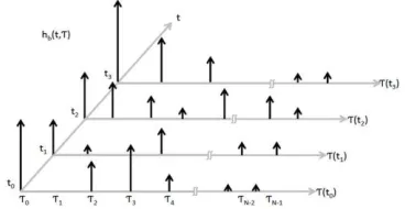
In an urban environment, the height of the mobile antennas is well below the height of the Surrounding structures. As a result, a Line of Sight (LOS) propagation path may or may not exist between the Base Station (BS) and the Mobile Station (MS). The radio waves transmitted from the BS, therefore, arrive at the MS after reflection, diffraction and scattering from the natural and man-made objects situated between the BS and the MS. The incoming radio waves arriving from different directions have different propagation delays. These multipath components, having randomly distributed amplitudes, phases and angles of arrival, combine vector ally at the receiver antenna causing the received signal to distort or fade. Thus, fading is the rapid fluctuations in the amplitude phase and the multipath delays of a radio signal over a short period of time so that large scale path loss effects can be neglected. Even when the MS is stationary, fading is caused by the movement of the surrounding objects. The changes in the environment or the motion of the MS result in spatial variations of amplitudes and phases manifest themselves as temporal variations. The mobile radio channel can be modeled as a linear filter having a time varying impulse response

h(t, )

The filtering nature of the channel is caused by the summation of amplitudes and delays of multiples arriving waves at the same instant of time.

Figure 5 : Time Varying impulse response of a multipath radio channel [1]

Problems in Cellular Mobile Communications:

In a cellular system interference is the major limiting factor in increasing capacity. Some of the interference sources are for example. Other base station transmitting in the same frequency band, another mobile user in the same cell, a call in progress in a neighboring cell, impairments caused by the propagation of radio waves, etc. as a result. Different types of system interference are yielded in the network. Among these interferences the most important are the following.

Co-channel interference (CCI)

This type of interference is caused by the interference between co-channel cells (cells with the same frequency channel) due to the frequency refuse. To reduce CCI, co-channel cells must be separated by a minimum distance to provide sufficient isolation due to propagation distance. Adjacent channel interference (ACI)

This other type of interference results when two frequency channels are adjacent in the frequency spectrum and one of them is leaking into the pass band causing interfering into the adjacent channel

ACI is mainly aggravated by imperfect receiver filters. This problem can be minimized with a careful filtering and channel assignments (assigning channels to a cell which is not adjacent in frequency).

Inter-symbol interference (ISI) When the signal travels through a channel, objects in transmission path can create multiple echoes of the signal. Whose occur at the receiver and overlap in successive e slots. This is known as inter-symbol interference equalizers at the receiver can be used to compensate the effect of ISI created by multi-path within time dispersive channels.

[image:4.612.76.260.586.681.2]

(5)

International Journal of Emerging Technology and Advanced Engineering

672 Thermal noise finally, the additive thermal noise is a factor that always corrupts a transmitted signal through a communication channel. Generally this thermal noise is assumed to be an additive white Gaussian noise (AWGN).

III. CHANNEL FADING TECHNIQUES

The physical medium between the transmitter and receiver is known as channel. This channel results in random delay (random phase shift) with total a factor. Channels may be three types

Type Description Examples

Simplex One way only FM radio, television

Half duplex Two way, only

one at a time

voice Radio

Full duplex Two way, both at the same time

Mobile systems

IV. TYPES OF SMALL SCALE FADING MODELS

There are many models that describe the phenomenon of small scale fading. Out of these models, Rayleigh fading, Ricean fading and Nakagami fading models are most widely used

Iv (A) Additive White Gussian Noise Model:

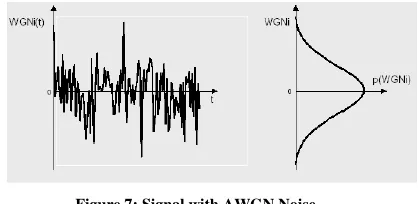
[image:5.612.339.548.414.516.2]

The simplest radio environment in which a wireless communications system or a local positioning system or proximity detector based on Time of- flight will have to operate is the Additive-White Gaussian Noise (AWGN) [4] environment. Additive white Gaussian noise AWGN) is the commonly used to transmit signal while signals travel from the channel and simulate background noise of channel. The mathematical expression in received signal that passed through the AWGN channel where transmitted signal is and is background noise An AWGN channel adds white Gaussian noise to the signal that passes through it. It is the basic communication channel model and used as a standard channel model. The transmitted signal gets disturbed by a simple additive white Gaussian noise process.

Figure 6 : Block diagram of AWGN Channel model The autocorrelation function of WGN is given by the inverse Fourier transform of the noise power spectral density AWGN(f):

The autocorrelation function is zero for t≠ 0. This means that any two different samples of WGN, no matter how close together in time they are taken, are uncorrelated. The noise signal WGN (t) is totally decor related from its time shifted version for any t≠0.

Figure.7: Signal with AWGN Noise IV(B) Rayleigh Fading Channels :

When information is transmitted in an environment with obstacles (Non Line-of-sight - NLOS), more than one transmission paths will appear as result of the reflections. The receiver will then have to process a signal which is a superposition of several different transmission paths. If there exists a large number of transmission paths may be modeled as statistically independent; the central limit theorem will give the channel the statistical characteristics of a Rayleigh Distribution (Fig 5)

(6)

International Journal of Emerging Technology and Advanced Engineering

673 Figure8 : Rayleigh distribution

Iv (C) Ricean Fading Model:

The Ricean fading model [6] is similar to the Rayleigh fading model, except that in Ricean fading, a strong dominant component is present. This dominant component is a stationary (non fading) signal and is commonly known as the LOS (Line of Sight Component).

V. DECISION FEED BACK EQUALIZER

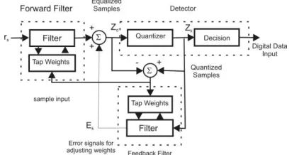
The basic limitation of a linear equalizer, such as transversal filter, is the poor perform on the channel having spectral nulls. A decision feedback equalizer (DFE) is a nonlinear equalizer that uses previous detector decision to eliminate the ISI on pulses that are currently being demodulated. In other words, the distortion on a current pulse that was caused by previous pulses is subtracted. Figure 7 shows a simplified block diagram of a DFE where the forward filter and the feedback filter can each be a linear filter, such as transversal filter. The nonlinearity of the DFE stems from the non linear characteristic of the detector that provides an input to the feedback filter. The basic idea of a DFE[7] is that if the values of the symbols previously detected are known, then ISI contributed by these symbols can be cancelled out exactly at the output of the forward filter by subtracting past symbol values with appropriate weighting. The forward and feedback tap weights can be adjusted simultaneously to fulfill a criterion such as minimizing the MSE. The DFE structure is particularly useful for equalization of channels with severe amplitude distortion, and is also less sensitive to sampling phase offset. The improved performance comes about since the addition of the feedback filter allows more freedom in the selection of feed forward coefficients.

[image:6.612.341.547.188.297.2]

The exact inverse of the channel response need not be synthesized in the feed forward filter, therefore excessive noise enhancement is avoided and sensitivity to sampler phase is decreased.

Figure 9: Decision feedback equalizer VI. ADAPTATION ALGORITHMS

This section briefly introduces two well-known algorithms that possess different qualities in terms of the performance i.e one is least mean square (LMS) and other is Recursive least square filter (RLS).

VI (A) Least mean square algorithm:

The least mean-square (LMS) algorithm [3, 8, 10] is probably the most widely used adaptive filtering algorithm, being employed in several communications systems. The LMS algorithm is a gradient-type algorithm that updates the coefficient vector by taking a step in the direction of the negative gradient [12] of the objective function, i.e.

Where μ is the step size controlling the stability, convergence speed, and misadjustment. To find an estimate of the gradient, the LMS algorithm uses as objective function the Instantaneous estimate of the MSE, i.e resulting in the gradient estimate

(7)

International Journal of Emerging Technology and Advanced Engineering

[image:7.612.65.269.155.295.2]

674 Table 1

The Least Mean Square Algorithm

LMS ALGORITHM

for each k

{

}

In order to guarantee stability in the mean-squared sense, the step size μ should be chosen in the range

Where tr{.} trace operator, and

is the input-signal autocorrelation matrix. The upper bound should be considered optimistic and in practice a smaller value is recommended [3].

The main drawback of the LMS and the NLMS algorithms is the slow convergence for colored noise input signals. In cases where the convergence speed of the LMS algorithm is not satisfying, the adaptation algorithms presented in the following sections may serve as viable alternatives.

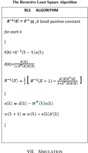
VI (B) The Recursive Least-Squares (RLS) Algorithm:

The RLS algorithm is a recursive implementation to overcome the problem of slow the least-squares (LS) solution, i.e., it Minimizes the LS objective function. The recursions for the most common version of the RLS algorithm, which is presented in its standard form in Table 1.2, is a result of the weighted least-squares (WLS) objective function

Differentiating the objective function with respect to and solving for the minimum yields the following

equation (i)]w(k)= )

Where 0 < λ ≤ 1 is an exponential scaling factor often referred to as the forgetting factor.

Defining the quantities

And =

the solution is obtained as

The recursive implementations is a result of the formulations

And

The inverse R−1(k) can be obtained recursively in terms of R−1(k−1) using the matrix inversion lemma1 [1]

Table 2

The Recursive Least Square Algorithm

RLS ALGORITHM

(I)

,

δ Small positive constant for each k

{ K(k) =

R(K)=

]

}

VII. SIMULATION

[image:7.612.351.534.332.649.2]

(8)

International Journal of Emerging Technology and Advanced Engineering

675 A. Linear Qualization for Frequency Flat Fading

(a) Begin with single-path, frequency-flat fading.

(b) The receiver uses a simple 1-tap LMS (least mean square) equalizer, which implements automatic gain and phase control.

(c) The script commadapteqloop.m runs multiple times

(d) Each run corresponds to a transmission block

(e) The equalizer resets its state and weight every transmission block. (To retain state from one block to the next, you can set the Reset Before Filtering property of the equalizer object to 0.)

(f) Before the first run, commadapteqloop.m displays the initial properties of the channel and equalizer objects

[image:8.612.354.537.148.280.2]

(g) The red circles in the signal constellation plots correspond to symbol errors. In the "Weights" plot, blue and magenta lines correspond to real and imaginary parts, respectively

Figure 10: BER & constellation equalized vs non- equalized B. Linear Equalization for Frequency-selective Fading

Simulate a three-path fading channel (frequency-selective fading)

(a) The receiver uses an 8-tap linear RLS (recursive least squares) equalizer with symbol-spaced taps.

[image:8.612.55.275.178.499.2]

(b) The simulation uses the channel object from

A

but with modified properties.

Figure 11 : BER & constellation equalized vs non-equalized C. Decision feedback Equalization (DFE) for

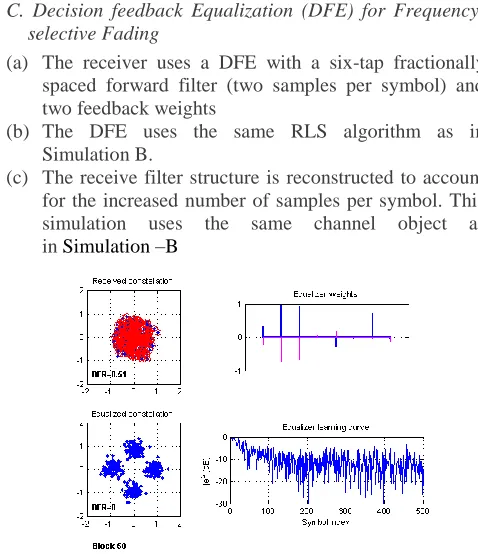
Frequency-selective Fading

(a) The receiver uses a DFE with a six-tap fractionally spaced forward filter (two samples per symbol) and two feedback weights

(b) The DFE uses the same RLS algorithm as in Simulation B.

(c) The receive filter structure is reconstructed to account for the increased number of samples per symbol. This simulation uses the same channel object as in Simulation –B

Figure 12: BER & constellation equalized vs non-equalized

[image:8.612.321.560.307.584.2]

(9)

International Journal of Emerging Technology and Advanced Engineering

676 COMPARISION TABLE: 3

VIII. CONCLUSION

It has been shown that relative performance of linear and decision feedback equalizers in both frequency-flat and frequency-selective fading channels. Simulations have shown that how a one-tap equalizer is sufficient to compensate for a frequency-flat channel, but that a frequency-selective channel requires an equalizer with multiple taps. Finally, it showed that a decision feedback equalizer is superior to a linear equalizer in a frequency-selective channel.

REFERENCES

[1] T. S. Rappaport, ―Wireless Communications: Principles and Practice‖, Second Edition, 2002

[2] J. G. Proakis, ―Digital Communications‖, Fourth Edition, 2001 [3] S. Haykin, ―Adaptive Filter Theory‖, Fourth Edition, 2002

[4] B. Sklar. Rayleigh Fading Channels in Mobile Digital Communication systems, Part I: Characterization. IEEE Common. Mag., 35(7):90–100, July 97.

[5] B. Sklar. Rayleigh Fading Channels in Mobile Digital Communication systems, Part II: Mitigation. IEEE Common. Mag., 35(7):102–109, July 97

[6] A. Alimohammad, S.F.Fard, B.F.Cockburn and C.Schlegal,―Compact Rayleigh and Rician fading simulation based on random walk processes‖, IET Communications, 2009, Vol.3, Issue 8, pp 1333-1342 Doubly Selective Channels. In IEEE Global Communicatio

[7] Vladimir D. Orlic, Miroslav Lutovac, ―A solution for efficient reduction of intersymbol interference in digital microwave radio,‖ Telsiks 2009, pp.463-464.

[8] P. S. R. Diniz Adaptive Filtering: Algorithms and Practical Implementations,Kluwer Academic Publishers, Boston, 1997 [9] I. Barhumi, G. Leus, and M. Moonen. Time-Varying FIR Decision

Feedback Equalization of nsConference, volume 4, pages 2263– 2268, San Francisco, CA USA, December, 1-5 2003

[10] B. Widrow and M. E. Hoff, ―Adaptive switching circuits,‖ IRE Western ElectricShow and Convention Record, pp. 96–104, August 1960

EQUALIZER channel AL GO

NO.OF WTS

RE CEI VE D BE R

EQ UA LIZ ED BE R

FREQUENCY FLAT

LINEAR RAYLEIGH LM S

1

.15

₀

FREQUENCY SELECTIVE

LINEAR RAYLEIGH RL S

8

.49 .49

FREQUENCY SELECTIVE

DFE RAYLEIGH RL

S

Performance Comparison of Linear and Decision Feedback Equalizers in Flat and Frequency Selective Fading Channel

International Journal of Emerging Technology and Advanced Engineering

Performance Comparison of Linear and Decision Feedback

Equalizers in Flat and Frequency Selective Fading Channel

Pradyumna Ku. Mohapatra

, Siba Prasad Panigrahi

, Jibanananda Mishra

International Journal of Emerging Technology and Advanced Engineering

International Journal of Emerging Technology and Advanced Engineering

International Journal of Emerging Technology and Advanced Engineering

h(t, )

International Journal of Emerging Technology and Advanced Engineering

International Journal of Emerging Technology and Advanced Engineering

International Journal of Emerging Technology and Advanced Engineering

,

]

International Journal of Emerging Technology and Advanced Engineering

A

International Journal of Emerging Technology and Advanced Engineering

1

0

8

[6 2]

₀