ISSN 1992 - 1950 ©2010 Academic Journals
Full Length Research Paper
Vehicle speed detection in video image sequences
using CVS method
Arash Gholami Rad
1,3*, Abbas Dehghani
2and Mohamed Rehan Karim
1 1Department of civil Engineering, University of Malaya. 50603 Kuala Lumpur, Malaysia.
2Department of Electrical Engineering, Sadjad Institute of Higher Education, Mashhad, Iran.
3Department of Computer Science, UCLA, 420 Westwood Plaza, Los Angeles, CA 90095, USA.
Accepted 5 November, 2010
Video and image processing has been used for traffic surveillance, analysis and monitoring of traffic
conditions in many cities and urban areas. This paper aims to present another approach to estimate the
vehicles velocity. In this study, the captured traffic movies are collected with a stationary camera which
is mounted on a freeway. The camera was calibrated based on geometrical equations that were
supported directly by using references. Camera calibration for exact measurements may be possible
while accurate speed estimation can still be quite difficult to achieve. The designed system has the
ability to be extended to another related traffic application. The average error of the detected vehicle
speed was ± 7 km/h and the experiment was operated at different resolutions and different video
sequences.
Key words: Vehicle speed detection, video sequence, computer vision, background modeling,
traffic
monitoring.
INTRODUCTION
The daily life of people encounters more problems as the
population continuously increases in urban area, and road
traffic becomes more congested because of high demand
and less level of road capacity and infrastructure. Since
the effects of these problems are significant in daily life, it
is important to seek efficient solutions to reduce them.
Vehicle speed detection is very important for observing
speed limitation law and it also demonstrates traffic
conditions. Traditionally, vehicle speed detection or
surveillance was obtained using radar technology,
particularly, radar detector and radar gun.
The radar system operation is known as Doppler shift
phenomenon. The basic concept about this system is
Doppler shift that happens when the created sound is
reflected off a moving vehicle and the frequency of the
returned sound is slightly changed. This method, with
spatial equations and equipments, obtains the speed of a
moving vehicle. However, this method still has several
disadvantages such as the cosine error that happens
when the direction of the radar gun is not on the direct
*Corresponding author. E-mail: [email protected]
path of the incoming vehicle. In addition, the cost of
equipment is one of the important reasons, and also
shading (radar wave reflection from two different vehicles
with distinctive heights), and radio interference (error
caused by the existence of similar frequency of the radio
waves on which a transmission is broadcasted) are two
other influential factors that cause errors for speed
detection and finally, the fact that radar sensor can track
only one car at any time is another limitation of this
method.
Many works and efforts have been done for vehicle
detection and speed measurements. Ferrier et al. (1994)
introduced vehicle detection based on frame difference,
un-calibrated camera (Pumrin and Dailey, 2002), motion
tra-jectories (Melo et al., 2006), geometric al optics
(Jianping et al., 2009), and digital aerial images (Fumio et
al., 2008; Wen and Fumio, 2009) are already introduced.
Also, Huei-Yung and Kun-Jhih (2004) used blur images to
find out the vehicle speed and Pumrin and Dailey (2002)
utilized camera motion detection for automated speed
measurements. Shisong et al. (2006) took advantage of
feature point tracking for vehicle speed measurements.
2556 Int. J. Phys. Sci.
Outstanding
reference
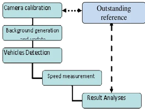
Figure 1. System architecture.
automatically detect vehicle speed in an accurate manner.
The algorithm needs only a single video camera and a
Cor2Duo computer possessor with Matlab software which
is installed on computer to operate the detection of the
vehicle. The procedure only requires installing the camera
directly above the roadway. The camera calibration which
is based on a geometrical and analytical model is simple
and is explained in the study. In addition, the calibration
does not require any information about the camera and
only the specification of the camera, like its frame rate
and frame size, which are obtainable through the
software, are essential.
MATERIALS AND METHODS
Here, another method to detect vehicle speed based on the camera coordination and calibration is proposed. First, the vehicle detection system architecture was described followed by a description of each component in the framework respectively.
Vehicle detection system architecture
In this paper, a new algorithm that utilizes the video image processing and camera optics to detect vehicle speed in precise manner is presented. The algorithm requires only a video camera and a computer and can concurrently detect vehicle speeds in different lanes with less than 7% error. The camera location must be set up over the surface of the road with its optical axis inclined downward to the roadway to cover the road plane.
Vehicle detection system architecture
[image:2.612.48.287.71.251.2]The software system is composed of 6 subsystems as shown in Figure 1, namely, the camera calibration unit, the background update and removal unit, the vehicle detection unite, the speed measurement unit, the result analysis unit and the outstanding reference. The result accuracy is compared with outstanding references which are the moving vehicles as we know the exact speeds of them that are driven by assistants during calibration.
Figure 2. The vehicles’ coordination in image.
Figure 3. Camera setting.
Camera calibration
Camera calibration is one of the important aspects of the study. The vehicles’ location in video images is 2-D (dimension), however, the vehicles in real world are 3-D, but because vehicles cannot leave the road surface, vehicles’ motion is also in 2-D (Figure 2) which makes the transformation of image coordinates and vehicles’ coordinates a 2D-to-2D mapping that can be precisely formulated. In this section, the calculation of the pattern function between vehicle coordinates in the image and real-world coordinates is performed. How the video camera is installed when the video images are captured from the road traffic and what characteristics are involved in that has to be determined. As shown in Figure 3, the camera is set at the height of H above the road surface with its optical axis sloped at an angle 1 from the road. The relation between camera lens angle and the domain covered by camera can be determined using geometrical equations.
Calculation of angle and perpendicular of vista
[image:2.612.325.570.74.257.2]×
=
2
3
tan
2
L
θ
P
(1)2 2
)
(
H
h
D
L
=
−
+
(2)=
P
2
3
tan
)
(
2
×
H
−
h
2+
D
2×
θ
(3)
Where: P is perpendicular field of view in the camera screen;
θ
3
is the angle view covered by the camera; H is the height of the camera; D is the horizontal distance between the camera and vehicles; h is the height of vehicles, and L is real distance between camera and vehiclesNote that if
θ
1
→
∠
90
°
thenL
→
D
and we can simplify the above equation to:
=
2
3
tan
2
D
θ
P
(4)Also, we can extract
θ
1
if we assume we do not have any vehicle which meansh
→
0
and we can write:=
H
D
arctan
1
θ
(5)and the angle for blind area is:
=
H
d
2
arctan
2
θ
(6)Where d2 is the blind area as shown in Figure 3. Also, we have:
1
3
2
2
1
3
θ
θ
θ
θ
θ
θ
=
−
→
=
−
(7)We can also find out the blind area which is equal to:
2
tan
)
3
1
tan(
2
H
θ
θ
H
θ
d
=
−
=
. (8) [image:3.612.304.571.76.251.2]Camera tendencies for three types of aerial images are shown in Figure 4. The bottom Images are the grids of section lines seen on different types of camera angle.
In this study, we calculate the vehicle speed as the vehicle enters the scene and passes two third of the road. The region at one third of the scene, which is located at the bottom of the image, is called detection region. In this case, when the vehicle arrives in the detection region, the vehicle centroid is near the middle of the image.
In this study, because the image height is 120 pixels and the detection region which is at the middle of the image is located 4 m from the bottom of the image, the length of each pixel is approximately 4/60 = 0.067 m. Therefore, we calibrate the camera and adjust the speed detection system with the well known vehicle with speed of 50 km/h and derive the calibration coefficient, which is the coefficient used to increase the accuracy of measurements.
High oblique
High oblique Low oblique
Low oblique
Figure 4. Camera tendencies and grid view results for vertical and oblique aerial images.
Moving vehicles and speed detection
The image processing in this study is an important task and another complex component. This task requires processing data such as the background extraction and removal, moving vehicle detection and localization, vehicle shadow removal, applying filter for image correction and calculation of the vehicles’ speed, etc.
The data captured through the video camera have a combination of consecutive image frames and each frame consists of numerical quantity of pixels which carry two types of data, background and foreground. The background contains the static objects such as parking vehicles, road surface and building or any other stationary objects and also climatic conditions and daylight/night time. The foreground represents moving objects such as pedestrians, moving vehicles or any other moving objects. In order to find out the speed of moving vehicles, the first step is to extract and remove the background. Therefore, the foreground which has the valuable data can be extracted and utilized for needed information such as speed, classification and number of the vehicles.
Background extraction
As aforementioned, background extraction and removal is one of the important parts of the vehicle detection that is highly applicable for the acquisition of foreground data. Moreover, if background image difference is used with no update of background image, this would lead to incorrect and unsuitable results. Therefore, the dynamic background extraction method which can estimate it while there are environmental changes in a traffic scene is required.
Background extraction algorithms are divided into several types. Ridder et al. (1995) used adaptive background estimation and foreground detection using kalman filter. Bailo et al. (2005) used background estimation with Gaussian distribution for image segmentation. Shi et al. (2002) introduced Adaptive Median Filter for Background Generation and Asaad and Syed (2009) utilized morphological background estimation.
[image:3.612.42.302.254.476.2]2558 Int. J. Phys. Sci.
( )
( )
j
t
f
t
k
jm xy n m n xy − = −
=
10 (9)
Where: n is frame number,;
f
xy( )
t
n is the pixel value of (x,y) inn’th frame;
k
xy( )
t
n is the pixel mean value of (x,y) in n’th frame averaged over the previousj
frames, andj
is the number of the frames used to calculate the average of the pixels value.Foreground extraction and vehicle detection applying CVS
Here, a method called combination of saturation and value or CVS is applied. Basically, the method which had been used for foreground extraction based on the frame difference is described as follows:
−
−
=
− −T
t
f
t
f
Background
T
t
f
t
f
Foreground
t
N
n xy n xy n xy n xy n xy)
(
)
(
0
)
(
)
(
1
)
(
1 1 (10)where,
N
xy(
t
n)
is the value of the foreground or background of the picture at pixel (x, y) in n’th frame and T is the threshold used to distinguish between the foreground and background.The disadvantage of this method is that a constant threshold is applied to all pixels and when objects are in low speed, the frame differences become small and therefore, using a low threshold can extract these foreground spots, but more background spots will be introduced than the foreground spots. On the other hand, a high threshold also will generate imperfect foreground detection. Moreover, the similar difficulty appears in the Gaussian foreground extraction, where standard deviation is utilized to determine the threshold and foreground spots may be miscalculated as background. In this paper, the CVS method is proposed to calculate foreground.
The important result that was founded in this study is, the color or hue is not affected in each frame and is almost constant but in the daylight alternation of the light intensity, it has been changed and has influence on the frames. Therefore, it is necessary to use effective and productive color model like HIS (Hue, Saturation, Intensity) model rather than RGB (red, green, blue) color spaces, but because HIS model is not defined in MATLAB software, we utilize HSV (Hue, Saturation, Value) Color Spaces instead of
HIS color spaces: The method as we proposed for object recognition is that first, the background is extracted based on value and saturation and then, it was subtracted from current frame which is also based on value and saturation and finally, the results were merged together. The flowchart is shown in Figure 9.
The proposed foreground detection method is based on value and saturation color space.
Edge detection and centered recognition
After foreground extraction, the collected images will transfer to binary image because the operations such as edge detection, noise and dilation removal and object labeling are suitable in binary platform.
SPEED DETECTION
The speed of the vehicle in each frame is calculated using the position of the vehicle in each frame, so the next step is to find out the blobs bounding box, and the centroid. The blob centroid is important to understand the distance of the vehicle moving in consecutive frames and therefore as the frame rate of captured moves is known, the calculation of the speed become possible.
This information must be recorded consecutively into an array cell in the same size as the captured camera image because the distance moved by the centroid is needed which is a pixel with a specific coordinate in the image to find out the vehicle speed. To find out the distance moved by the pixel, suppose the pixel has the coordinate like:
( )
a
b
i
=
,
i
−
1
=
( )
e
,
f
,where the centroids location is showed in frame i and i-1 for one vehicles, with (a, b) coordinate and (e, f) coordinate.
The distance difference for the vehicle is equal to:
2 2
1
(
a
e
)
(
b
f
)
d
=
−
+
−
. (11)and if the image sequence is 25 frames per second, the time between two consecutive frames is equal to 0.04 s and finally the speed can be determined from the equation:
t
x
K
V
∆
∆
=
. (12) Where K is the calibration coefficientRESULTS
Here, we explain our accomplish result step by step and
at first, the results for background generation using mean
filter method as previously explained had been shown in
Figure 5 .
In the next step, the background extracts in two modes,
one with advantage of saturation (Figure 7) and the other
is based on value (Figure 8).
The next step for foreground extraction and vehicle
detection need to subtract background with current
image .As shown in Figure 6, for moving object detection
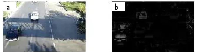
based on value, the object with white and bright color is
recognized explicitly but the vehicle with dark color is not
recognized as well as we expect. In order to resolve this
issue and recover this miscalculation, we used the
second and third character of HSV model which is
saturation and value. The Saturation base extraction for
extracting foreground is utilized and as shown in Figure
10, the dark vehicle is illuminated but the object with
bright color cannot be extracted.
These two methods can be combined to reveal both
dark and light colored vehicles (Figure 11) and the vehicle
velocity can be determined based on introduced
calibration.
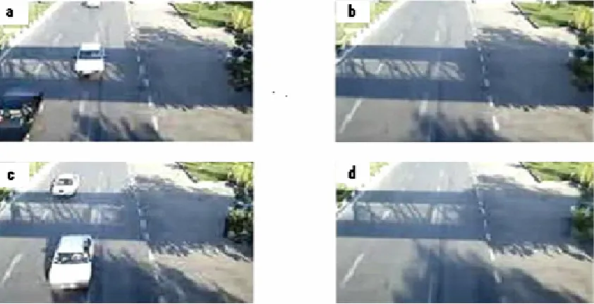
Figure 5. Result of background extraction. (a) video frame number 22; (b) background frame number 22; (c) video frame number 30; (d) background frame number 30.
[image:5.612.101.522.76.292.2]Figure 6. Moving object detection based on value. (a) video frame number 22, (b) moving object based on value.
Figure 7. Background based on saturation.(a) video frame number 22, (b) frame based on saturation, (c) background based on saturation.
[image:5.612.147.472.351.438.2] [image:5.612.70.543.497.576.2] [image:5.612.73.543.633.711.2]2560 Int. J. Phys. Sci.
Video image sequence
Pre processing
Current image based on saturation
Current image based on value
Background extraction and update
Based on
saturation Based on value
Vehicle detection
based on saturation Vehicle detection based on value
+
_
_
+
+
Foreground [image:6.612.153.469.74.478.2]detection
Figure 9. The flowchart of foreground detection.
Figure 10. Moving object detection based on Saturation. (a) Video frame number 22, (b) moving object based on saturation.
Morphological operations are used generally for the
object structure improvement (convex hull, opening,
skeletonization, closing, thinning, object marking), image
preprocessing (shape simplification, ultimate erosion,
noise filtering), segmentation of object and measurement
of area and perimeter (Sonka et al., 1999).
[image:6.612.148.474.529.629.2]Figure 11. Moving object detection based on saturation and value. (a) Video frame number 22(b) moving object based on saturation and value.
[image:7.612.142.477.73.162.2]Figure 12. Noise and dilation removal. (a) The moving object, (b) Binary image, (c) After noise removal and filling holes.
Figure 13. The bounding box and the centroid. (a) Video frame number 45, (b) Bounding box and the centroid in frame number 45, (c) Video frame number 51, (d) Bounding box and the centroid in frame 51.
which commonly happen during the image and video
processing and cause disorder and error in the final step
which is the obtaining of traffic information.
The dilation is used for examining and expanding the
shapes in the input image to extend the border of the
regions of moving objects. Foreground pixels enlarge
while holes within those areas become smaller. On the
other hand, erosion erodes the border of the foreground
pixels and the boundaries of moving objects become
smaller in size and shape, and the holes turn into greater
size and quantity. An opening is the dilation of the erosion
of an object boundary by a chosen structural element. A
closing is the reverse act of an opening and the basic
functionality of this operation is the noise removal. The
main effect of opening is to remove small objects from the
foreground which are not really moving objects and set
them to background, while closing removes small holes
inside moving objects (Figure 12).
Finally for speed detection as we proposed, the
bounding box and the centroid are specified and shown in
two consecutive frames in Figure 13.
[image:7.612.141.473.362.535.2]2562 Int. J. Phys. Sci.
Table 1. The experimental results of the speed detection system
Real speed (Km/h) 1
X
(pixel) (x, y)2
X
(pixel)(x, y)
∆
x
=
X
1−
X
2(pixel)x
∆
(m) Error
System detection speed (Km/h)
40 (64,76) (74,69) 12.2 0.81 0.03 38.6
50 (63,47) (79,42) 16.76 1.12 0.01 50.4
60 (64,79) (85,84) 21.58 1.44 0.07 64.7
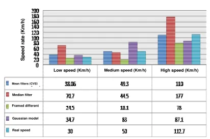
Mean filters (CVS) Median filter Framed different
Gaussian model
Real speed
Low speed (Km/h) Medium speed (Km/h) High speed (Km/h)
S
pe
ed
r
at
e
(K
m
/h
)
Figure 14. Experimental results of the speed detection system with different background models.
system are shown and the error is calculated. In this
study, time intervals for speed detection are the same,
and equal to the difference of the time of two successive
frames, which is:
08
.
0
04
.
0
2
×
=
=
∆
t
s.
The error is calculated by comparing between the system
speed detection and the real speed which is obtained
from a reference vehicle.
As is shown in Table 1, the error occurs because of two
reasons, first, as a result of the non linearity in grid
oblique shown in Figure 4 and second, because of
erosion and dilation which still have effects even after
morphological operation.
DISCUSSION
Our purposed speed detection system works fairly
accurately to measure different speeds but it is sensitive
to the threshold, and the threshold must be adjusted to a
proper value. Spatially, when it is needed to convert HSV
images to binary ones it has to carefully be considered,
otherwise the system has high error. Another thing that
needs to be discussed is that the speed detection system
normally gives good results in compression with other
background models.
We test our system with different speed level and
different background models shown in Figure 14. The
testing speed, 30, 50 and 112.7 (km/h) which are real
speeds and the results of the speed detection system for
each background model are shown.
Conclusion
[image:8.612.103.515.183.456.2]extraction and speed recognition. In the first step, the
mean filter method for background generation that was
one of the effective ways for background extraction was
used. In the second step, a novel algorithm which takes
advantage of the two-color based characteristics and
combines them for object extraction is introduced. This
approach is more robust against misdetections and the
problem of the merging or splitting of vehicles and finally,
in the third step, the vehicle speed is determined. The
approach used is not affected by weather changes.
Vehicle extraction and speed detection had been
imple-mented using the MATLAB software. The prototype can
process around 12 frames per second on a core2Duo
processor at 2 GHz.
REFERENCES
Asaad AMA, Syed IA (2009). “Object identification in video images using morphological background estimation scheme” Chapter, 22: 279-288.
Bailo G, Bariani M, Ijas P, Raggio M (2005). ”Background estimation with Gaussian distribution for image segmentation, a fast approach,” Proc. IEEE Intl. workshop on Measurement Systems for Homeland Security, Contraband Detection and Personal safety, pp. 2-5. Ferrier NJ, Rowe SM, Blake A (1994). Real--time traffic monitoring. In
WACV94, pp. 81—88.
Fumio Y, Wen L, Thuy TV (2008). “Vehicle Extraction And Speed Detection From Digital Aerial Images” IEEE International Geosciences and Remote Sensing Symposium, pp. 1134-1137. Huei-Yung L, Kun-Jhih L (2004). “Motion Blur Removal and Its
Application to Vehicle Speed Detection”, The IEEE International Conference on Image Processing (ICIP 2004), pp. 3407-3410.
Jianping W, Zhaobin L, Jinxiang L, Caidong G, Maoxin S, Fangyong T (2009). “An Algorithm for Automatic Vehicle Speed Detection using Video Camera” Proc. IEEE 4th Int. Conference Comput. Sci. Educ., pp. 193-196.
Melo JN, Bernardino A, Santos-Victor AJ (2006). Detection and classification of highway lanes using vehicle motion trajectories, IEEE Trans. Intelligent Trans. Syst., pp. 188- 200.
Pumrin S, Dailey DJ (2002). “Roadside Camera Motion Detection for Automated Speed Measurement”, the IEEE 5th International Conference on Intelligent Transportation Systems”, Singapore, pp. 147-151.
Ridder C, Munkel O, Kirchner H (1995). Adaptive background estimation and foreground detection using kalman-filter, Technical report, Bavarian Research Center for Knowledge-Based Systems. Shi P, Jones EG, Zhu Q (2002). “Adaptive Median Filter for Background
Generation - A Heuristic Approach,” Proceedings of the International Conference on Imaging Science, Systems, and Technology CISST '02, Vol. 1, CSREA Press, pp. 173-179.
Shisong Z, Toshio K (2006). “Feature Point Tracking for Car Speed Measurement”, the IEEE Asia Pacific Conference on Circuits and Systems (APCCAS 2006), pp. 1144-1147.
Sonka M, Vaclav H, Roger B (1999). ”Image Processing, Analysis, and
Machine Vision”
http://portal.acm.org/author_page.cfm?id=81100646621&coll=GUIDE &dl=GUIDE&trk=0.