Does the type of diffuser matter?

(1)

Does the type of Diffuser matter?

Author: William Fehlhaber Supervisor: Prof. T. Cox

Co-supervisor: Prof. I. Drumm

@00271181

School Computing, Science, and Engineering College of Science and Technology University of Salford, Salford, UK

(2)

Abstract

A study was conducted to see how different diffuser designs affected the acoustic

(3)

List of Figures

2.1 FDTD Diagram (from Cox [2004] and [Schneider, 2013]) . . . 10

3.1 The threshold of disturbance for separate signals as a function of delay time and amplitude. From [Kuttruff, 2009] . . . 19

3.2 Armin Van Buuren’s private studio (From [Senior, 2009]) . . . 20

3.3 Air Studio’s Studio 2 at Lyndhurst Hall (From [Air, 2015]) . . . 21

4.1 Flat Panel Reflection . . . 27

4.2 Triangular Diffuser Reflection . . . 28

4.3 Convex Diffuser Reflection . . . 28

4.4 This figure shows the temporal response and narrow band frequency response of the Flat Panel. . . 29

4.5 This figure shows the temporal response and narrow band frequency response of the Triangular Diffuser. . . 29

4.6 This figure shows the temporal response and narrow band frequency response of the Convex Diffuser. . . 30

4.7 This series of images shows the interaction of a cylindrical wave with a Schroeder Diffuser. . . 30

4.8 Schroeder Geometry Temporal and Frequency Response . . . 31

4.9 Convex Diffuser . . . 32

4.10 Concave Diffuser . . . 33

4.11 Triangular Diffuser . . . 34

4.12 Triangular Diffuser Construction [Left Side] . . . 34

4.13 Triangular Diffuser Construction [Right Side] . . . 35

4.14 Curved Diffuser from Frequency Modulation . . . 36

4.15 Schroeder Diffuser . . . 38

5.1 This image illustrates the Anechoic Simulation Setup. The red region outlines a basic area where a diffuser geometry would be tested. . . 39

5.2 This figure is an illustration of the set-up method for Experiment 2. An exam-ple diffuser geometry is shown in red. The absorbing boundaries are shown in green. The tested sources are shown in pink. The various dimensions are marked accordingly. . . 41

(6)

5.4 This is a view of the scale model with all treatments secured [Outside] . . . 43 5.5 This is a view of the inside of the scale model with no treatment. This is done

to convey an understanding of how the construction is pieced together. . . 43 5.6 These are the tested orientations used in each test. Only the Concave Diffuser

is shown here however, this same orientation method translates for the other diffuser models as well. Moving clockwise from the top left, these orientations are designated as: x-horizontal/y-horizontal, x-horizontal/y-vertical, x-vertical/y-horizontal, and x-vertical/y-vertical. . . 44

6.1 This is the polar response plot of the flat panel in an anechoic environment. The black lines in the first column show the response of the 1/3rd octave band centred at 1 kHz. The red lines in the second column show the response of the 1/3rd octave band centred at 3 kHz. The blue lines in the third column show the response of the 1/3rd octave band centred at 5 kHz. The first row shows the results of the tests for the source at 0◦ (on axis). The second row shows the results of the tests for the source at +30◦ off axis. The third row shows the results of the tests for the source at 60◦ off axis. . . 46 6.2 This group of colormaps display the results of the flat panel in an anechoic

environment. Each colormap is a test for a given source position. In other words, Flat Panel 0◦ shows the results of the flat panel at 0◦ on axis. The z-axis (color axis) is in Pascals. . . 47 6.3 This group of colormaps display the results of the Convex Diffuser in an anechoic

environment. Each colormap represents a test for a given source position. The z-axis (color axis) is in Pascals. . . 48 6.4 This group of colormaps display the results of the Concave Diffuser in an anechoic

environment. Each colormap represents a test for a given source position. The z-axis (color axis) is in Pascals. . . 49 6.5 This group of colormaps display the results of the Triangular Diffuser in an

ane-choic environment. Each colormap represents a test for a given source position. The z-axis (color axis) is in Pascals. . . 50 6.6 This group of colormaps display the results of the FM Diffuser in an anechoic

environment. Each colormap represents a test for a given source position. The z-axis (color axis) is in Pascals. . . 51 6.7 This group of colormaps display the results of the Schroeder Diffuser in an

ane-choic environment. Each colormap represents a test for a given source position. The z-axis (color axis) is in Pascals. . . 52 6.8 These are the schroeder curves for the Flat Panel, Convex Diffuser and Concave

Diffuser. Each line plot uses a separate coloured line for each source position. . . 53 6.9 These are the schroeder curves for the Triangular Diffuser, FM Diffuser and

(7)

6.10 3rd octave frequency response of the room with the source at 0◦Normalized to˙ the 3rd octave frequency response of the source function. . . 55 6.11 3rd octave frequency response of the room with the source at 30◦Normalized to˙

the 3rd octave frequency response of the source function. . . 56 6.12 3rd octave frequency response of the room with the source at 110◦Normalized to˙

the 3rd octave frequency response of the source function. . . 56 6.13 This is the 3rd octave band frequency response for the different orientations with

the source position at source 0◦ (on axis). Red represents the triangular diffuser. Green represents the convex diffuser. Blue represents the concave diffuser. The response is normalized in order to remove the response of the transducer. . . 58 6.14 This is the 3rd octave Band frequency response for the different orientations with

the source position at source +30◦ (off axis). Red represents the triangular dif-fuser. Green represents the convex difdif-fuser. Blue represents the concave difdif-fuser. The response is normalized in order to remove the response of the transducer. . 59 6.15 This is the 3rd octave band frequency response for the different orientations with

(8)

Acknowledgements

I would like to thank Trevor Cox and Ian Drumm for their assistance over the course of this project. Their knowledge and guidance has helped me gain a better understanding of

(9)

Introduction

The manipulation of reflections in order to change perceptual acoustic characteristics, is a central topic in room acoustics. Diffusers are commonly employed in order to control

reflections, reduce colouration and minimize the intensity of echoes. In concert hall acoustics, they may be used for envelopment purposes, while in a studio, they may be used to reduce image shift for accurate monitoring and reproduction. While what diffusers “do” is well defined by a collection and consensus of experimental data and practical application, there are still many topics in active discussion. What diffuser designs are right for a specific task? Do some diffusers sound better than others?

The main goal of this research is to explore the effect of diffusers in the context of small rooms using the Finite Difference Time Domain method and a scale model. The numerical method allows for the observation of wave propagation in a given environment. Data can be collected for further manipulation from either the whole field or at specific points.

The use of simulation of acoustic environments in order to accurately predict performance is of key importance to civil planners, architects, acoustic consultancies and design firms. Simulation can help to solve problems in existing spaces by allowing users to recreate an environment and find solutions to a problem in a cost effective manner. This is especially important in critical listening environments such as studios and concert halls where the cost of trial and error is too high.

The ultimate question is: Does the type of diffuser matter? This report hopes to answer the question by simulating certain diffuser geometries in a given studio configuration. Questions that will arise include:

1. What determines if a specific diffuser is more effective than another?

2. Are there any design compromises or limitations that must be considered?

3. Does orientation matter?

This report is divided into separate sections that will guide the reader through the relevant fundamental concepts of acoustics in order to understand how these are applied and

(10)

numerical modelling methods and why Finite Difference Time Domain was chosen for this research. The chapter also shows how the derivation from the previous chapter is changed to finite difference form. Chapter 3 outlines basic principles of room acoustics and the various sources of room colouration. The chapter then extends to a discussion of studio design and what was chosen for this project. Chapter 4 outlines the principles of diffuser design and which geometries were tested in this research. Chapter 5 gives a description of the experiments conducted and Chapter 6 illustrates the data and includes analyses of the resulting data. Chapter 7 is the conclusion and gives a summation of the results and some implications. This report does not include a dedicated literature review as the relevant

(11)

Chapter 1 Basic Acoustics

There are a variety of texts that outline the relevant topics for this project however, the relevant physics to create the appropriate simulation is narrow in scope and non-debatable. Therefore, the review of the necessary literature for this section is brief.

Heinrich Kuttruff’s academic text “Room Acoustics” [Kuttruff, 2009] offers thorough introductions to the immediately useful concepts of wave propagation. The first chapter discusses the wave equation and the physics behind wave propagation.

The Stanford Exploration Project [Sepstanford.edu, 2000] hosts a web page that outlines the derivation of the acoustic wave equation. This is the derivation used in this section as it is the most thoroughly explained derivation. Suzanne Fielding offers a full lecture listed as “The basic equations of fluid dynamics” [Fielding, 2007] which demonstrates the meaning of continuity of mass in fluid dynamics which is essential when deriving the wave equation.

1.1 Wave Equation

When a sound wave propagates through a medium, the particles of the medium, such as air, undergo vibrations about their mean positions in space. This travelling wave changes the localised density of molecules that make up that medium. The areas where molecules are more compressed are known as compressions and the areas where molecules are less dense are known as rarefactions. Once the wave has passed, the displaced particles move back to their original positions. Consequently, the variations of both pressure and velocity occur as

functions of both time and space, the expression of which is known as the wave equation.[Burg et al.] [Kuttruff, 2009] [Everest and Pohlmann, 2009]

(12)

mass, m, will undergo acceleration, a, if there is an applied force, F.

F =ma (1.1)

The force arises from pressure differences, P, at opposite sides of the small volume as the wave propagates through the medium. The acceleration is the change in velocity, ~u, over a period of time which means we can express the Newtonian Law as:

∂P

∂x =−ρ ∂ux

∂t (1.2)

The second physical process is the conservation of mass which is expressed as Cox and D’Antonio [2009] Fielding [2007]:

∂P

∂t =−K ∂ux ∂x (1.3) -or-∂ux ∂x = 1 −K ∂P ∂t (1.4)

This equation means that the change in pressure, P, is in proportion to a property of the medium called incompressibility K. ~u is the particle velocity and the subscript denotes the dimension.cis the speed of sound in the medium and, ρ, is the density of the medium.

K =ρc2 (1.5)

The following set of equations will derive the wave equation from equations 1.2 and 1.3. The first step is to apply the spatial derivative, _∂x∂ , to the conservation of momentum, equations 1.2. This yields:

∂2P

∂x2 =−ρ

∂2ux

∂t∂x (1.6)

The second step is to apply the temporal derivative, _∂t∂, to the conservation of mass, equations 1.3. This yields:

∂2_P

∂t2 =−K

∂2_u

x

∂t∂x (1.7)

Substituting equation 1.6 into 1.7 yields:

∂2P ∂t2 =K

1 ρ ∂ ∂x ∂P ∂x (1.8)

Which is the wave equation:

∂2_P

∂t2 =c 2∂2P

∂x2 (1.9)

In order for this form of the wave equation to be true, then a few assumptions must be made. These include but are not limited to:

(13)

2. The fluid is irrotational.

3. There are no viscous forces.

4. The disturbance from the wave propagation is small.

5. The medium is homogeneous.

(14)

Chapter 2 Finite Difference Time Domain

Finite Difference Time Domain (FDTD) is a numerical technique that was proposed by Kane Yee in 1966 [Yee, 1966]. It offers a procedure for discretising the differential form of the wave equation as given in the previous chapter. This chapter begins with the formulation of the wave equation for two dimensions and explains the general method of how this equation will be applied for simulation. The chapter then proceeds to transform the wave equation into finite difference form. The chapter then continues to explain the advantages and

disadvantages of FDTD as compared to other numerical techniques. There are key ideas to understanding Finite Difference Time Domain for use in acoustics.

Firstly, it is best to begin with an understanding of how FDTD is formulated. Compact FDTD methods tend to be distinguished by their method of spatial discretisation. Spatial discretisation is important because it allows the finite difference form of the equation to be solved. The method of meshing is also important because it can help describe the boundaries of a volume more accurately while offering more points to represent a wave front. A

simplification of the effect of doing so is that the method of spatial discretisation determines the relative phase velocity of the medium for wave propagation along the axis of those degrees of freedom [Kowalczyk and Van Walstijn, 2010]. Relative phase velocity is an important consideration because it determines how fast a wave will travel at a given frequency in that medium. To be clear, this is an error, and the change in relative phase velocity is greatest along the axis of those degrees of freedom. There are methods and algorithms proposed that can help nullify the effects of this at added computational cost and time. The resulting dispersion error of this change in phase velocity can be redistributed as more degrees of freedom are added. [Kowalczyk, 2008].

(15)

the method chosen for this simulation.

However, it is not enough to consider solely which formulation would be used. While it is the most important starting point, it is also important to consider the method of computation. John B. Schneider’s academic text [Schneider, 2013] is focused towards electro-magnetic wave simulation however, Chapter 12 is dedicated to acoustics and simulating acoustic wave

propagation. This text offers insight to making a simulation scalable as well as improving code in order to make it distributable for parallel computation. There is nothing to debate in this text as it is not focused on the exploration of certain utilizations of FDTD. The main value lies in the procedures and methods offered for creating a simulation that runs efficiently. Schneider’s paper details the technical aspects for writing a FDTD simulation including how to quantify error, the max usable frequency of a simulation and how to troubleshoot common stability issues [Schneider, 2013].

As this paper investigates the acoustic behaviour of small rooms, it is important to account for different boundary conditions. Reflections from boundaries of an acoustic space play a pivotal role in room acoustics, however different materials and wall constructions yield different reflection behaviours. Real boundaries yield frequency-dependant conditions and therefore the formulation for that given material should include a frequency-dependent, complex wall impedance [Kowalczyk, 2008].

A common practice for simulating the effects of real materials is through the use of FIR filter networks [Botteldooren, 1995] [Huopaniemi et al., 1997]. A secondary method is through the use of convolution. Both of these methods can increase computation time dramatically. Convolution is a computationally demanding method to implement. There is also the issue that there is a difficulty of validation as full bandwidth data of a boundary’s impedance or a material’s absorptive properties are rarely available as well as time consuming to produce [Jeong, 2010]. The other problem with the practical implementation of a convolution

algorithm is that not all convolution algorithms are capable of being distributed on a GPU for computing. However, this is only an issue if you plan to port your program to other systems that may not have a GPU.

These considerations lead to another set of questions: How can one decide which materials to simulate (and provide a valid mathematical formulation) for a given experiment? Will the use of modelled boundaries offer any greater insight into the behaviours of diffusers, the resulting reflections or their implementation in a given small room? The next paragraph aims to guide why modelled boundaries were not used.

(16)

3D model (which was beyond the capability of the available computer). Lastly, the modelling of boundaries is unlikely to effect the utility of the general information from the simulations. One can still gain directivity information as well temporal and frequency information for any given point on the grid. However, one cannot just assume rigid boundaries. Therefore, a Perfectly Matched Layer (PML) is implemented for anechoic conditions and surface admittance is a purely real value that is adjusted to simulate non-rigid boundaries.

In summary, while none of these research papers discuss simulating diffusers or the results of diffusers, these papers do outline the considerations and decisions required in order to plan a FDTD simulation. Firstly, all of the following FDTD simulations used in this experiment are two dimensional, meaning only one plane of propagation is observed. The chief reason is that the computational capability of the available computer was limited. It did not have enough RAM to run a three dimensional simulation to the required resolution. Therefore, the

diffusers were designed to reflect along a single plane and only required one plane of analysis. Secondly, the original two degree of freedom algorithm, as proposed by Kane Yee, was chosen as it is most widely available for retesting. Thirdly, all simulations were run at a resolution at 400 nodes per metre in order to simulate to a high frequency and create negligible dispersion error and minimize geometry discretisation errors. Lastly, no specific surfaces were modelled for the boundaries. However, anechoic conditions are simulated using a Perfectly Matched Layer (PML) and surface admittance is adjusted to simulate non-rigid boundaries. Both of these conditions may be non-physical but, they do not interfere with the ability to analyse diffuser behaviour.

2.1 Expansion to Two Dimensions

In Finite Difference Time Domain, a field is discretised into a finite number of coordinate points to form a grid with a finite step size between each point. The most fundamental form of FDTD, uses a grid for the pressure field P , which is offset both spatially and temporally from a field for particle velocity ~u. When space and time are discretised into this field, future field values can be solved for in terms of known past field values. Figure 2.1 illustrates the basic concept [Cox, 2004] [Schneider, 2013].

In the figure, i is an index for the x direction and j is an index for the y direction. In order for this method to work, the step sizes ∆xand ∆y must be equal. ux and uy are the velocities for the x and y axes.

(17)

[image:17.595.123.475.63.345.2]

Figure 2.1: FDTD Diagram (from Cox [2004] and [Schneider, 2013])

Newtons Law in Equation 1.2 can be described for two dimensions as:

− ∂P

∂x =ρ ∂ux

∂t (2.1)

−∂P

∂y =ρ ∂uy

∂t (2.2)

The conservation of mass in Equation 1.3 can be described for two dimensions as:

∂P

∂t =−K

∂ux ∂x + ∂uy ∂y (2.3)

Therefore, the two dimensional wave equation is:

∂2_P

∂t2 =c 2

∂2_P

∂x2 +

∂2_P

∂y2

(2.4)

2.2 Wave Equation in Finite Difference Form

As stated earlier, the sound pressure P and particle velocity ~u make up the grid in Figure 2.1. BothP and~uare functions of time and position and therefore the equations used to represent this must include:

Pn+

1 2

i,j =P

i∆x, j∆y,

n+1 2

∆t

(18)

un_x_i,j =ux

i+1 2

∆x, j∆y, n∆t

(2.6)

un_y

i,j =uy

i∆x,

j+1 2

∆y, n∆t

(2.7)

The variables ∆xand ∆y represent the spatial step size for the x and y while i and j

represent the appropriate indexes. ∆t is the temporal time step and n is the respective index. The update equations come in the form of [Cox, 2004] [Sepstanford.edu, 2000]:

Pn+

1 2

i,j =P n−1

2

i,j −K∆t

ux

i+ 1₂,j −uxi−1

2,j

∆x +

ux

i+ 1₂,j −uxi−1

2,j

∆y

!

(2.8)

un_x+1

i+ 1₂,j =u

n x

i+ 1₂,j −

∆t ρ





Pn+

1 2

i+1,j−P n+1₂

i,j ∆x



 (2.9)

un_y+1

i,j+ 1₂ =u

n y_{i,j+ 1}

2

− ∆t

ρ





Pn+

1 2

i,j+1−P

n+1₂

i,j

∆y )



 (2.10)

The temporal step size, ∆t:

∆t =

s c

q

( 1 ∆x)

2_{+ (} 1 ∆y)

2

(2.11)

s is the Courant Number and is given in the following equation. It is a necessary number for solving Finite Difference equations as it defines the relationship between temporal step size and spatial step size [Schneider, 2013]. If a wave is propagating across a discretised field, its amplitude needs to be computed at discrete time steps of equal duration and this duration must be less than the time for the wave to travel to adjacent grid points. For this two dimensional case, s must satisfy:

s ≤ c∆t

∆x + c∆t

∆y (2.12)

This expands out as more degrees of freedom are computed.

In a discrete simulation, the smallest possible wavelength must have at least 2 samples per period. However, the number of samples necessary to describe a single wavelength with reduced error is actually closer to 10 nodes per wavelength [Schneider, 2013] and there is a direct connection with the spectral resolution of the analysed signal. Therefore, the maximum frequency fc is given as:

fc= 1

(19)

2.3 Non Rigid Boundaries

A default FDTD model has rigid terminations which means that any acoustic simulation would have an infinite reverberation time. This is not useful for simulating believable rooms and therefore, the boundaries of a room should be able to reflect sound and simulate the loss of energy whether that is by transmission or absorption.

This can be accomplished by implementing the following set of variables at the terminations of the grid. B is the normalized surface admittance and is a real value. [Cox and D’Antonio, 2009] [Kuttruff, 2009]

Z is the surface impedance.

Z = ρc

B (2.14)

R is the reflection coefficient. The reflection coefficient is usually a complex value because there are changes in the amplitude and phase of the components of the wave. However, the values used in this experiment are real values for the sake of simplicity. [Everest and

Pohlmann, 2009] [Kowalczyk, 2008]

R= (Z −(cρ))

(Z + (cρ)) (2.15)

α is the absorption coefficient.

α= 1−(|R|)2 (2.16)

These equations change for sound at oblique incidence. However, using this simplified

approach does not affect the utility of the information about the behaviour of diffusers, which is the purpose of this project. Furthermore, there is no reason why the diffusers themselves cannot be considered absolutely rigid during the simulations.

2.4 Anechoic Terminations

For free field simulations there are a number of methods that can be used to implement anechoic conditions. Firstly, the variable α from the previous section can be changed to a value close to 1. This will give near anechoic conditions. However, a more common method is to implement a Perfectly Matched Layer (PML).

(20)

Absorption for each node is introduced such that:

αi =α

xi

xP M L

2

(2.17)

The maximum absorption for 1/10 of the PML is:

α = 1

Kδtln(10) (2.18)

The update equations in 2D for the PML area are:

Pn+

1 2

i,j =P n−1

2

i,j e

−Kαδt₋ 1−e−Kαδt

Kα K ux

i+ 1₂,j −uxi−1

2,j

∆x +

ux

i+ 1₂,j −uxi−1

2,j

∆y

!

(2.19)

un_x+1

i+ 1₂,j =u

n x

i+ 1₂,je

−Kαδt₋ 1−e

−Kαδt

Kα





Pn+

1 2

i+1,j−P n+1₂

i,j

ρ∆x



 (2.20)

un_y+1

i+ 1 2,j

=un_y

i+ 1 2,j

e−Kαδt− 1−e

−Kαδt

Kα





Pn+

1 2

i+1,j−P n+1₂

i,j

ρ∆y



 (2.21)

There are only 3 update equations. There should be at least 2 per boundary (one for pressure and one for the particle velocity along the relevant axis). However, this is really an issue of indexing and is up to the individual program but, the update equations are similar.

2.5 Pros and Cons of Finite Difference Time Domain

In acoustics, the Finite Difference Time Domain method is primarily used to model wave propagation in acoustic environments. As a mesh structure, interference and diffraction are inherently modelled [Kowalczyk, 2008]. As a time domain technique, FDTD can be used to analyse a single frequency or a broad bandwidth with a single simulation. For example, if a pulse is used as a source function, then the response of the system over a wide bandwidth can be obtained through the use of a single simulation [Schneider, 2013]. This is useful when attempting to acquire the impulse response of a room for auralisation purposes while

accounting for the dispersion characteristics of rooms or objects with complex geometries or material properties. Another powerful feature of FDTD is that it can be used to simulate time variant systems such as structures that change in shape, as well as changing source or receiver positions. Lastly, solving for higher-order reflections does not increase the memory load for a given simulation time and resolution. Regardless, there are a variety of drawbacks with FDTD.

(21)

When the field is discretised, the phase velocity of the wave differs from the phase velocity of the modelled medium [Kowalczyk and Van Walstijn, 2010]. This causes high frequencies to travel at different speeds than lower frequencies. This is known as dispersion error and is not only frequency dependant but also directionally dependant. The original staggered grid method mentioned above is the original method proposed by Yee and is the method used in this simulation. However, it yields only first order accuracy and exhibits its strongest

dispersion error along the x and y directions [Kowalczyk, 2008].

There are two ways to overcome this:

1. The user can change the method to use a higher order partial differential to redistribute the dispersion error or another FDTD scheme. However, deriving the update equations for a higher order partial differential is not an easy task and will create more multiply add operations which will make the simulation slower [Kowalczyk, 2008] [Botteldooren, 1995] [Schneider, 2013].

2. If another method is not chosen, the user must “over-discretise” or “over-sample” the field. The issue with this choice though is that it will increase computation time and memory consumption dramatically [Kowalczyk, 2008].

When describing complex geometries the grid must have a sufficiently small spatial step size in order to accurately describe the smallest geometric feature of an object. The larger the grid or the higher the resolution, the longer the simulation takes to run and the more memory that is required for the calculation. However, the relationship between the computational resources required and the resolution is linear. That is to say:

• For one dimension of propagation when the resolution is doubled for a given problem, the memory required and computation time are also doubled (2x).

• For two dimensions of propagation when the resolution is doubled for a given problem, the memory required and computation time are increased by 4x .

• For three dimensions of propagation when the resolution is doubled for a given problem, the memory required and computation time are increased by 8x .

2.6 Other Mathematical Models

(22)

In Ray Tracing models, the principles of geometric optics are applied to approximate the path of propagation of an acoustics wave. There are some key challenges that face such a

simulation. Firstly, sound has a significantly longer wavelength than light and so small objects have little effect on an acoustic wave but diffraction effects, when they do occur, are significant [Kufner, 2008]. Secondly, modelling the relative phase of waves at a specific

receiver position is important and is effected by the characteristics of the boundary. The main benefit of Ray Tracing is that it can be used to model all surface geometries and scattering effects. However, the computational requirements increase with the demand to compute higher order reflections. These disadvantages mean that Ray Tracing is usually only valid for approximating the behaviour of an environment at higher frequencies.

The Boundary Element Method (BEM) is another technique of solving the wave equation. The BEM provides a solution by combing boundary integral equations and the Finite Element Method in order to discretise the surface and describe its acoustic characteristics. The BEM can be used to efficiently discretise a complex surface geometry for modeling. Like FDTD, the BEM can be used to model the entire range of human hearing provided that the mesh size of discretisation is significantly smaller than the wavelength of the highest frequency required.

However, there is a key disadvantage: BEM gives rise to fully populated matrices and

(23)

Chapter 3 Basic Room Acoustics

This research is chiefly concerned with the implementation of diffusers in small rooms. This chapter will open with a statement of the relevant literature pertaining to a variety of topics in room acoustics and will then continue to introduce acoustic phenomena in small rooms and the different perceptual effects that may be created. The last section of the chapter will describe different small room designs and how these designs differ.

It may be best to begin with the basic concept that room acoustics is chiefly concerned with the propagation of waves in a confined volume of air. There are several objective parameters that are used to describe the performance of a room. The most fundamentally measurement is the impulse response of the room. From that measurement one can extract the

reverberation time, RT60, as well as the reverberation time of different frequency bands and the frequency response of a room at a given receiver position [Rossing, 2007]. This research is concerned with the response at the listening position in a studio environment.

Other subjective and objective parameters that can be extracted from the impulse response include Clarity, Sound Strength, Spaciousness [Rossing, 2007]. However, these parameters (as well as others) are not as useful in this context because they require an integration time of 80 milliseconds. Sound will travel a path distance of roughly 27 metres which means that most reflections will likely arrive back to the listening position in a small room in that time. Due to this, the basic analyses mentioned in the previous paragraph will form the extent of the data compared.

However, there is some objective data known about how human hearing works that may indicate if there are possible perceptual effects when comparing simulated rooms. Chapter 7 of Kuttruff’s text [Kuttruff, 2009] opens with the idea that the acoustic designer has to find ways to meet the expectations of the average or listener for whatever space it is. In section 7.2 he discusses the conditions which lead to the perceptibility of reflections. He presents data that dictates: The threshold of perception for a reflection with a 50 ms delay changes

(24)

humans are less sensitive to reflection interference when listening to music rather than speech. Further within the same chapter, Kuttruff defines that perceptibility of a reflection is a

function of both delay time and level [Kuttruff, 2009]. These points are discussed in greater detail within the chapter.

Besides perceptual effects, there is the main topic which is the design of the room itself. There are some practical considerations when dealing with small rooms for production purposes. It is not unusual for a modern professional studio to be expected to produce

content for a number of formats including mono, stereo, and surround as well as Dolby Atmos in the near future. At this time Dolby Atmos is more common for use in dubbing theatres and block buster film post production. This research tests the results of a 5 point surround system. There are a few accepted general designs that are discussed later in this chapter. However, the main concern is that these methods were intended for stereophonic reproduction [Walker, 1995] [Walker, 2007]. This predicament is a central topic that this research does not address and could be greatly aided by.

The stereophonic reproduction has generated few fairly stabilised and accepted principles of design such as a reflection free zone in front of the room, the Live End-Dead End principle, left-right symmetry of the monitoring room, symmetrical placement of the Left and Right loudspeakers. The stereophonic design principles do not directly extend to multichannel reproduction, and the current lack of clear design approach is generating a lot of debate. [Varla et al.]

3.1 Acoustic Phenomena in Small Rooms

(25)

3.1.1 Room Modes

Room modes are a number of resonances that exist in a constrained volume when the medium (air) is excited by a source (speaker). Room modes are the result of standing waves that occur when half the wavelength (and multiples of that wavelength) of a signal is equal to a dimension of propagation within the room. There are well established methods for calculating the modal frequencies of cuboid rooms. However, the important point is that all rooms are finite bodies and all finite bodies resonate. The larger the room, the longer the wavelength for the fundamental frequencies. In small rooms such as studios and listening rooms,

fundamental resonant frequencies are likely to lie within the range of human hearing.

Modal phenomena yields some perceptual effects. The magnitude of modal frequencies is likely to be increased and as this is the resonant frequency of the volume of air, the decay time for these frequencies is increased. This gives the perception of a room having a tonal characteristic [Kuttruff, 2009] [Cox and D’Antonio, 2009]. It is possible to create a diffuser that is large enough to affect room modes, but this is not practical and so room modes are not relevant to the typical bandwidth of diffusers.

3.1.2 Colouration and Echo

Colouration is defined as changes in timbre. Timbre is the perceptible attribute of a signal which enables an observer to judge that two non-identical sounds, having the same loudness and pitch, are dissimilar. Timbre depends primarily upon the waveform, but also upon the sound pressure and the temporal aspects of the signal [Rubak, 2013].

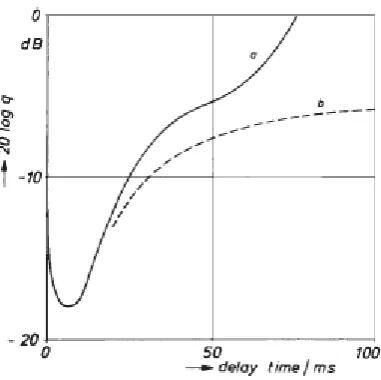
A source of colouration is caused by the interference between the direct and reflected sounds. If a reflected sound combines with the direct sound under 50 ms, the human ear acts as a short time integrator. This integration behaviour restricts the ability to resolve successive acoustic events that happen within that time frame and therefore, humans perceive the tonal characteristics of the signal. The threshold of colouration (Figure 3.1) is shown as a function of delay time and amplitude [Kuttruff, 2009].

The threshold is lowest (most disturbing) when the delay is between 1 ms and 25 ms but rises (less of a problem) when the delay time is above 25 ms. Between 25 ms and 50 ms the

perception of colouration turns into a perception of rough successive events. This is

(26)

[image:26.595.194.385.66.256.2]

Figure 3.1: The threshold of disturbance for separate signals as a function of delay time and amplitude. From [Kuttruff, 2009]

3.2 Studio and Listening Room Design

There is a standard set by the International Telecommunications Union for how to design a listening room environment for experimental work. Rec.ITU-R BS.1116-1 [ITU, 1997]

proposes that “the use of standardized methods is important for the exchange, compatibility and correct evaluation of the test data”. The standard then goes on to outlines a number of features that of the room construction that must be validated by measurement. The standard lists a number of considerations governing reverberation time tolerances, the operational room response curve and room dimensions. According to Rec.ITU-R BS.1116-1, the following room dimension ratios should be observed to ensure a reasonably uniform distribution of the room modes:

1.1w

h ≤ l

w ≤4.5 w

h −4 (3.1)

where l is the length, w is the width, andh is the height of the room.

R. Walker had illustrated that, for a given room volume, it is possible to plot the modal variation or distribution for different room ratios [Acoustics.salford.ac.uk, a]. The analysis showed that there were only a few room ratios that could be applied to a range of room volumes. However, there is more than the one outlined by the ITU standard.

Furthermore, there are some other limitations. Both analyses are only applicable to

(27)

[image:27.595.146.449.117.319.2]

walls and partitions as not every room is perfectly rectangular [Acoustics.salford.ac.uk, a] [Varla et al.] [Walker, 1995].

Figure 3.2: Armin Van Buuren’s private studio (From [Senior, 2009])

Listening room environments and studios that actually meet this exact specification are not common. If a business were to require a space for sound reproduction purposes, such as a studio, then that business must be located in an area with enough potential traffic in order to generate the revenue to operate. Typically, this means an urbanized environment. In a city, the ability to acquire the real estate to develop an already existing space is expensive enough. The likelihood of finding a space of these exact proportions as well as acquiring the rights to develop, severely hamper the ability to create rooms to this standard. Therefore, most

businesses tend to retrofit the rooms they have available. To illustrate this point, both Figure 3.2 and Figure 3.3 display the main monitoring and mixing environments used by

professionals. Neither of these rooms fit the ITU standard completely.

Due to the many constraints hobbyists and businesses have to work with, the ITU standard is used more as a set of guidelines and Rec.ITU-R BS.1116-1 includes a notice that states “This Recommendation forms the base reference for the other Recommendations, which may

contain additional special conditions or relaxations of the requirements included in this Annex” [ITU, 1997]. Therefore, there are some broader goals designers try to achieve when creating a monitoring environment for studios.

Most studio designs try to achieve the following broader aspects [Errede, 2015]:

• The room should be acoustically isolated. This is not simulated and is assumed.

(28)

[image:28.595.149.449.54.357.2]

Figure 3.3: Air Studio’s Studio 2 at Lyndhurst Hall (From [Air, 2015])

basis of many standards.

• The reverberation time (RT60) should be under 0.5 seconds.

• The frequency response of the room should be relatively even. This means that room modes should be controlled with resonant absorbers and speaker and listening positions should be positioned accordingly. This also means that colouration effects due to

reflection interference should be reduced either through the use of diffusers or broadband absorption.

To be clear; a room that meets these goals can be achieved if one follows the guidelines set out by the ITU standard. However, there is a lack of flexibility in the ITU standard that hampers its application to most situations. To address this problem, there are a number of different studio room configurations that have been formulated over previous decades, however, only two will be described.

3.2.1 Live End Dead End

(29)

or cause image shift.[Cox and D’Antonio, 2009]

This design is flexible as it can be used to treat rooms of irregular geometries as well as smaller rooms. However, it is usually only used for mono and stereo monitoring. This is partly due to the fact that during its inception, most audio was consumed in the form of stereo recordings. However, surround sound systems of 5.1 are becoming increasingly popular due to developments in the video game industry and a developing independent film industry with lower budgets. Therefore, despite this design not being the most effective, it is still common for project use.

However, this design suffers from acoustics that vary widely throughout the space. This design also requires that the room is perfectly symmetrical about the listening axis and offers a small listening position. This design also requires a minimum room size to control the effects of interfering reflections and requires significant absorption even at lower frequencies.

3.2.2 Reflection Free Zone and Controlled Image Design

A Reflection Free Zone (RFZ) is a method of addressing room acoustics created in the 1980’s. The design creates a spatial and temporal reflection free zone surrounding the listening

position. The zone is spatial, because it only exists within a certain area of the room; and it is temporal, because the interfering reflections are only controlled over a certain window of time [Cox and D’Antonio, 2009] [Walker, 2007]. Essentially, the boundaries of the room are angled in order to reflected sound away from the listening position to create a longer mean free path for the wave to travel[Fazenda and Angus, 2002]. However, this prediction typically only holds true at higher frequencies. The terminating or rear wall surface is comprised of absorbers and diffusers.

The Controlled Image Design (CID) is a similar method created in the 1990s by Bob Walker [Walker, 1995]. It also uses angled boundaries to lengthen the path of propagation like the RFZ but does not employ the use any absorbers. This means that CID’s require large amounts of space and have not been used outside of the BBC or major production facilities.

Neither of these designs are flexible or cheap to implement. They have certain size

(30)

3.2.3 Test Studio Design

The small room environment simulated in this experiment is a Live End Dead End Model. This was done because the design of a RFZ or CID usually employs the use of geometric simulations. These tools were simply not available. Furthermore, the scale model that was available was cuboid in shape and fitting an RFZ or CID within it would have greatly limited the available testable bandwidth as well as increasing costs of testing.

(31)

Chapter 4 Basic Principles of Diffusers

An acoustic diffuser is an acoustic treatment that is used to spread sound evenly through a space. This chapter will establish the basic principles of diffusers and diffuser operation. The chapter will then proceed to offer a detailed explanation for each diffuser design used in the following experiments. There are some key ideas and literature that may help guide an understanding of acoustic diffusers and why these designs were chosen.

There are a wide range of acoustic diffusers available in the market that come in a variety of geometries, sizes and materials for consumer and professional applications. The

implementation of these diffuser types can yield praise or criticisms. While there are

comments on the aesthetic appeal of certain designs, some critics say certain designs sound better than others or that there are correct ways of applying said designs. This is well summarised by Trevor Cox [Cox, 2004]:

“Informal conversations with practitioners have indicated that diffusers, either the presence or lack of them, are sometimes cited as reasons for the acoustics of a space failing to meet expectation. It is hard to know how much weight to put on these opinions, because they are usually not borne out by psychological

measurement using test juries and following scientific methods, but are simply individual opinions, albeit from recognised experts.”

Further confusion arises due to manufacturers who market their products with extraordinary claims that simply cannot be true and are not backed by measurement results.

(32)

may cause certain subjective descriptions of the space such as “spaciousness” and the removal of echoes. However, relating “global” descriptive coefficients to diffusers is difficult [Cox and D’Antonio, 2009].

A relevant paper is “The Analysis of Several Diffusers in a Reverberation Chamber by FDTD Method” by Baoli, Wu, Benqing and Shiming. The paper aimed to quantify if different diffusers are more effective in creating a diffuse field by looking at field uniformity in a simulated reverberation chamber. However, there is limited context given in the paper. The paper dictates little about the conditions of the environment including reverberation time. The conclusion stated that “it is found that the diffusers have good characteristics to enhance the reflected field and we can obtain better homogeneous field by reasonable arrangement of diffusers”[Baoli et al., 2002]. Unfortunately, what is reasonable was never clearly discussed. Also, these simulations were used to understand reverberation chambers and not small rooms with absorption and diffusion.

Coefficients are useful as they can be used to clearly evaluate and rank diffusers in an easily measurable and reproducible way [Cox and D’Antonio, 2009]. Two common coefficients used in diffuser design are the scattering coefficient and diffusion coefficient. Changing coefficients may simplify the optimisation of their design for a specific scenario as well as facilitate their input into geometrical models.

The scattering coefficient is intended to provide a simplified understanding of how much energy is removed from the specular direction. The specular component is the proportion of energy which is reflected in the same way as would happen for a plane surface [Cox and D’Antonio, 2009]. The scattered components give the energy reflected in a non-specular manner. This coefficient is also frequency dependent. The diffusion coefficient is a single figure that states the amount of diffuse reflections that can be expected for a given frequency band at a single source position [Cox and D’Antonio, 2009]. While a diffuser yielding

temporal spreading may yield a stronger diffusion coefficient, there is not a direct correlation between the spatial and temporal responses that can be gathered by the diffusion coefficient alone. Therefore, it is not compatible in geometric modeling methods. [Redondo et al., 2007] [Cox et al., 2015]

...We must note however that the frequency variability of the time-space spreading relationship implies that any projected relationship between ISO and AES results is likely to be complex (see for instance [50]), and that the main reason for

differences in results using the two standards is that the diffusion coefficient (see equation (15)) has a tendency to underestimate the spatial spreading. [Redondo et al., 2007]

(33)

”Contrasting surface diffusion and scattering coefficients” which was given at the 17th ICA, Italy in 2001. This paper is cited in this paper as [Cox and DAntonio, 2001].

The idea of temporal redistribution is an important facet that is discussed in greater detail, with examples, later in this chapter. To be put simply, it is the property that allows for the diminishing of comb filtering due to interference. However, there are unresolved questions. Do these coefficients translate directly to a change in some physical or measurable objective characteristics? Does this objective characteristic create a consistently observable or

noticeable subjective change? The experiment involved in this research may shed some light as to how complex these relationship may be while not offering a final resolution.

... preliminary results concerning the time domain features of the sound reflected by three different surfaces have indicated that FDTD can be useful for the

evaluation of sound diffusers in terms of time-spreading. Further research must be carried out in this area, to build a knowledge (objective and subjective) of the ability of sound diffusers to spread sound in time in addition to their well-known spatial spreading, towards a global time-frequency parameter to quantify

scattering. [Redondo et al., 2007]

4.1 Diffuser Operation

As the name would imply, diffusers are acoustic devices that aid in the process of diffusion. Broadly speaking, a diffuser has a given geometry that breaks an incident wave front and reflects the components of that wave front in many directions. It is well understood, and easy to visualise, that when a wave is incident upon a smooth flat surface, there is only one

reflected wave. If the incident wave strikes a corrugated surface, more reflected waves are produced. However, not all corrugated surfaces are diffusers.

In order to understand diffuser design, it is useful to define what the ideal acoustic diffuser is. The ideal acoustic diffuser will reflect an incident wave in all directions equally for all

frequencies at any angle of incidence.

The core principles of diffuser operation relate to the fundamental considerations of wavelength and object diffraction.

• At low frequencies when the wavelength of the sound is much larger than the dimension of the surface irregularity, or object, then the wave diffracts around the object.

• When the wavelength of the sound is similar to the dimensions of the surface

(34)

radiates sound back into the field. The resultant pressure distribution depends on the relative phase and magnitude of all waves received.

• At high frequencies, the scattering can be calculated by considering the surface to be a series of smaller plane surfaces. At this scale, Snell’s Law can be accurately applied. If the angle of incidence equals the angle of reflection, specular reflection will result.

The fundamental principles of diffraction tell us the very simple fact, that diffusers are band limited devices. There will be a lower limiting frequency which usually controls the depth of corrugations and this is often a starting point for diffuser design. Before exploring different diffuser designs, it is best to know how a basic geometry interacts with a wave in order understand what characteristics designers are trying to avoid.

Figure 4.1 illustrates a cylindrical wave reflected from a planar rigid surface. Upon reflection, the wave simply changes direction and results as specular reflection. The reflected wave is essentially unaltered meaning that none of the wavefront was reflected in another direction as all components of that wavefront are still in phase. In a room such as a studio, this reflection could be perceived as colouration which would make accurate sound reproduction difficult as it would interfere with the direct sound from whatever monitoring method was used.

Figure 4.1: Flat Panel Reflection

The next step is to create another simple surface that can be used as a diffuser. If one combines two flat panels, a triangle is achieved. Triangles can come in all manners of angle combinations however, the following set of images (Figure 4.2) illustrates a wave incident upon an obtuse triangle.

If one continues to add vertices, then a curved surface can be achieved. Figure 4.3 illustrates the effects of a cylindrical wavefront approaching and interacting with a convex curved surface.

In the case of both the triangular and curved simple surfaces, the reflections that result, may be distributed spatially or directed towards another area in the field. However, there are some other flaws with each design. In the case of the triangle, if the wavefront was incident

(35)

Figure 4.2: Triangular Diffuser Reflection

Figure 4.3: Convex Diffuser Reflection

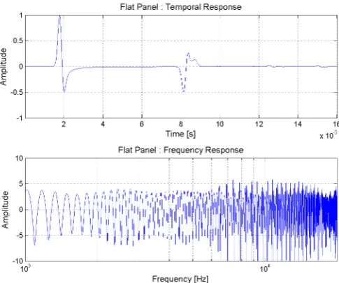
However, when the angle of incidence is 0◦on axis, the reflection along that same axis is severely attenuated. Upon adding more vertices to create a curved surface, the reflected wavefront is more bowed and the sound is more spatially distributed. In the case of the curved surface, it is generally safe to assume that this behaviour would persist across a wide range of angles of incidence. However, both simple geometries have the same fundamental problem as the flat panel. The pressure of the reflected wavefronts are negligibly different from the incident wavefront. If the reflected wavefronts were to arrive at a listening position, the reflection could be perceived as colouration with a comb filtering effect. To prove this point, the following set of figures (Figures 4.4 - 4.6 ) show the temporal response and a narrow-band frequency response of each basic animation.

(36)

[image:36.595.173.416.62.265.2]

Figure 4.4: This figure shows the temporal response and narrow band frequency response of the Flat Panel.

Figure 4.5: This figure shows the temporal response and narrow band frequency response of the Triangular Diffuser.

then the direct sound, the comb filtering effects are not as exaggerated. Comb filtering is an undesirable effect especially in small critical listening environments such as studios because the spectral content of the source cannot be perceived accurately.

[image:36.595.171.417.342.546.2]

(37)

[image:37.595.172.416.62.266.2]

Figure 4.6: This figure shows the temporal response and narrow band frequency response of the Convex Diffuser.

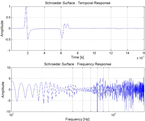
Figure 4.7: This series of images shows the interaction of a cylindrical wave with a Schroeder Diffuser.

The basic operation and design of a Schroeder diffuser will be discussed in the next section. However, this demonstration shows that a Schroeder diffuser creates a more intricate

interference pattern upon reflection. The temporal response illustrates that at a specific receiver point, the reflection is really a number of delayed reflections with varying phase relationships. This results in a frequency response that is less representative of a comb filter especially at higher frequencies.

The results of these basic demonstrations illustrate that there is more to a diffuser design or choice than simply its spatial scattering behaviour. There is also temporal scattering

behaviour that is necessary to consider. However, it may be a mistake to think of the Schroeder diffuser as “another surface” because a Schroeder diffuser is, essentially, an

(38)

[image:38.595.172.416.62.265.2]

Figure 4.8: Schroeder Geometry Temporal and Frequency Response

and how are still unanswered. Furthermore, these opening demonstrations take place in a free field environment. They are not indicative of the much more complex behaviour of scattering exhibited by more complex diffuser surfaces or real rooms with added boundaries and surface orientations.

4.2 Diffuser Designs

This section will give a brief overview of the surfaces used for each simulation. A reason will be given for their selection as well as basic design criteria. These diffusers were not chosen to test particular existing products or designs. They were simply chosen to offer a broad

comparisons between different geometries in order to gain insight to the behaviours of these objects. In total six surfaces are tested.

4.2.1 Flat Panel

A flat panel is included for every simulation. While not acting as a control, it forms some basis for comparison. This is done in part because, the spatial and scattering behaviours of flat panels are well understood and some reasonable assumptions can be made as to what should be expected. This panel is not angled in any way so the animations from Figure 4.3 represent the method of implementation used (flat against a boundary). The dimensions of the simulated panel are listed in the table.

(39)

4.2.2 Convex Diffuser

Some authors claim that convex cylindrical devices offer astounding diffusion characteristics. This is where Alton Everest and Ken C. Pohlmann’s [Everest and Pohlmann, 2009] text disagrees with Cox and DAntonio [Cox and D’Antonio, 2009]. This idea is not completely the case as clearly demonstrated in the section above. However, the last section ended with the idea that effective diffusers are arrangements of simple component geometries. Following that thought, we can ask: What happens when convex cylinders are arranged to form more

complex poly-cylindrical diffusers? Is the reflection a more intricate interference pattern or can we simply expect more of the same?

Length 2.40 metre

Diameter of Large Pipe 0.80 metre Diameter of Medium Pipe 0.55 metre

Diameter of Small Pipe 0.25 metre

The design of this diffuser is based off of actual sizes of materials that could be found for the scale model. The full scale dimensions of the simulated diffuser are listed in the table. The poly-cylinders are arranged by decreasing diameter from a central larger poly-cylinder. Each poly-cylinder is exactly half of a cylinder. Figure 4.9 displays an image of the model.

Figure 4.9: Convex Diffuser

4.2.3 Concave Diffuser

The Master Handbook of Acoustics claims that concave surfaces are to be avoided at all cost when controlling reflections in a room. It is logical to assume that at higher frequencies, the wave will be brought to a focus at some point away from the curve as dictated by

(40)

still has modern relevance when designing parabolic microphones.

Length 2.40 metre

Diameter of Large Pipe 0.80 metre

Diameter of Medium Pipe 0.55 metre Diameter of Small Pipe 0.25 metre

In diffuser design, if the focus is too close to the listening position (which is a reasonable risk to assume in small rooms) then the reflection may be perceived to be louder then the direct sound. However, does that dictate that the concave shape should be avoided entirely? What if that focus is moved to within the curve or close to the device? If one was to follow this logic, which is based off of the assumption that we can equate the behaviour of sound to rays of light, then is not reasonable to expect dispersion beyond the focal point?

[image:40.595.226.365.416.553.2]

The design of the concave diffuser used in this project should, in theory, exploit that. The arrangement is essentially, the inverse of the convex diffuser. Therefore, the focus should be at the “face” of the device. The full scale dimensions of the simulated diffuser are listed in the table while Figure 4.10 displays an image of the model.

Figure 4.10: Concave Diffuser

4.2.4 Triangular Diffuser

Arrangements of triangles have been sought for use as diffusers as well. With so much possible variation, the geometry of a triangle or pyramidal shape can offer a wide variety of scattering behaviours. Depending on the angle of incidence to the face of a triangle (or set of triangles), a wave can be reflected to the an angle far off axis or specularly.

(41)

arrangement. The dimensions of the full scale simulated diffuser are listed in the table. Figure 4.11 displays an image of the model.

Length 2.850 metre maximum Depth 0.475 metre

Figure 4.11: Triangular Diffuser

4.12 - 4.13 show the angles and measurements of the components of the triangular diffuser for reconstruction purposes.

(42)

Figure 4.13: Triangular Diffuser Construction [Right Side]

4.2.5 FM Diffuser

The FM Diffuser is not representative of any established diffuser design. The purpose of this design is to find out how large curved surfaces interact with a wave in a small room. This kind of geometry is typical of optimized curves, bi-radial and bi-cubic designs. To be clear, this curve can be recreated by the following set of values:

fa= 1.0Hz (4.1)

fb = 0.75Hz (4.2)

a= 0.4 (4.3)

b= 1.2 (4.4)

a is equal to half of the diameter of the large central pipe of the curved diffuser times scaling.

b is equal to half of the overall size of the other diffuser configurations. This is done for scaling purposes.

yb =bsin((fb2pi)t); (4.5)

ya=asin((ybfa2pi)t); (4.6)

(43)

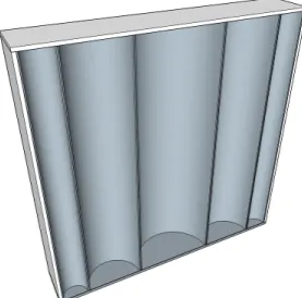
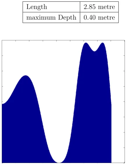
The dimensions of the simulated diffuser are listed in the table. The following figure 4.14 displays a cross sectional image.

[image:43.595.176.393.116.400.2]

Length 2.85 metre maximum Depth 0.40 metre

Figure 4.14: Curved Diffuser from Frequency Modulation

4.2.6 Schroeder Diffuser

A Schroeder Diffuser consists of a series of wells of the same width but different depths. The wells are separated by thin fins so that plane wave propagation will dominate within the wells. Ideally, these fins are infinitely thin and rigid and the depths of the wells are determined by a number sequence such as a quadratic residue sequence or primitive root sequence.

As the wavefront enters each well, it travels at the same speed but for different distances. The sound wave takes time to propagate in and out of wells, causing sections of the reflected wave to be delayed. The resulting interference pattern of the reflected wave is more complex

because all of these waves have similar magnitude but different phases. Therefore, the polar distribution of the reflected pressure is determined by the choice of well depth and the original wavefront is redistributed temporally.

The Schroeder Diffuser used for testing is based off of N = 43. N must be prime for the design to operate correctly. The design wavelength λ0 = 0.4 metres which corresponds with

(44)

the well width used here is 5 cm.

Most Schroeder Diffusers are only built with a N = 7 to N = 13 range. The reason is because Schroeder diffusers require precision during construction. Every component must be planar and every fitting must be square while maintaining structural integrity. For most situations, this does not present an issue as the diffusers are smaller as they are designed for a higher frequency (shallow depth) or are used in conjunction with duplicate diffusers. However, duplicate diffusers can yield periodicity effects which lead to uneven scattering of a sound wave. The design in this experiment is N = 43 because the diffuser needs to cover the same surface area of the wall as the other designs while still maintaining a reasonable well width. The periodicity effects should be avoided as this would complicate the comparison against the other surface designs.

The sequence sn is determined by:

sn =n2moduloN (4.8) For a N = 43 sequence this yields:

sn = ( 1, 4, 9, 16, 25, 36, 6, 21, 38, 14, 35, 15, 40, 24, 10, 41, 31, 23, 17, 13, 11, 11, 13, 17, 23, 31, 41, 10, 24, 40, 15, 35, 14, 38, 21, 6, 36, 25, 16, 9, 4, 1, 0)

To determine the well depths, dn, sn is inserted into:

dn =

snλ0

2N (4.9)

The following figure 4.15 displays a cross sectional image of the result of the sequence with fins inserted.

Therefore if the wells are 5 cm and the fins are 1 node. Then the dimensions should be as listed in following table.

Length 2.85 metre

(45)

[image:45.595.178.394.291.508.2]

(46)

Chapter 5 Experimentation Methods

5.1 Experiment 1: Simulated Free Field Test

[image:46.595.120.424.369.678.2]

This simulation is devised in order to understand the dispersion characteristics of diffusers in isolation.

Figure 5.1: This image illustrates the Anechoic Simulation Setup. The red region outlines a basic area where a diffuser geometry would be tested.

(47)

The source is placed along an arc around the diffuser. This distance is l+ 2 where l is the length of the diffuser in metres. The source positions tested are at 0◦ (on axis), +30◦, +45◦, +60◦ and +90◦. There are 180 receiver positions arranged along an arc at a radius ofl+ 1. The Courant Number is 0.707. The resolution for this grid is 400 nodes per metre which yields a sampling rate of 274560 Hz. The highest resolvable frequency of this simulation is 27456 Hz. Again, the oversampling is done to minimize the effects of dispersion error and geometry discretisation error.

Each geometry is tested for one source position at a time, therefore, there are 5 tests per diffuser design. For the sake of simplicity, the surface of the diffuser is assumed to be rigid so the surface impedance is infinite. Each simulation will use a Gaussian Pulse to deliver a wide bandwidth signal from the source positions. This means that each simulation will collect 180 impulse responses. From these tests, we hope to understand:

• How does a specific diffuser geometry scatter sound spatially?

• How does a specific diffuser geometry scatter sound temporally?

• How does this scattering behave over a number angles of incidence?

5.2 Experiment 2: Simulated Room Test

This simulation is devised in order to understand the effect of the diffuser designs in an example small room. The chosen scenario is illustrated in Figure 5.2. It consists of a 5.1 monitoring system in a Live End Dead End Room with a width of 4.35 m and a length of 9 m. The absorbing regions are shown as green and the diffusers are red. The green areas correspond with an absorption coefficient, α, of 0.7. The sources (pink) are arranged around the listening position in a circle with a 1 m radius. Due to the fact that the room is

symmetrical, only half of the source positions are necessary for each test.

Only one source position is used for each test, in other words, combined source position responses are not tested. Again, the simulation is run at a resolution of 400 nodes per metre. The simulated time is 0.4 seconds. Each simulation will provide a room impulse response at the listening position. From these tests, we hope to understand:

• Do the effects of these different diffuser designs yield a difference beyond a 3 dB threshold?

(48)

Figure 5.2: This figure is an illustration of the set-up method for Experiment 2. An example diffuser geometry is shown in red. The absorbing boundaries are shown in green. The tested sources are shown in pink. The various dimensions are marked accordingly.

A 3dB threshold is used because this is the threshold for a single specular reflection. The paper titled ”The sensitivity of listeners to early sound field changes in auditoriums” attempted to answer what characteristics could be used to measure the perceptual

characteristics of diffusers used in concert halls. Unfortunately, some measurements were not applicable to this study, such as Clarity Index because they require the use of an 80ms

integration window. This is not really feasible in small rooms because, as stated earlier, most reflections will arrive within the first few milliseconds. The paper [Cox et al., 1993] was not able to find a threshold for diffuse reflections. This is possibly due to the fact that diffuse reflections are not like specular reflections in that there will be masking between octave bands due to the different delayed reflections with different relative phases.

5.3 Experiment 3: Scale Model Room Test

The previous experiments are only two dimensional even though humans observe and interact with the physical world in three dimensions. It is possible to create a 3D FDTD simulation. However, this was not done and the reasons are explained in the section labelled Further Work.

Scale models are a well established method of testing theoretical room designs. They are typically used when planning concert hall acoustics which means the scale is typically around 1:20. Not only is the geometry of the room smaller by scale but the wavelength is also

Does the type of diffuser matter?