Relative effects of statistical preprocessing and postprocessing on a regional hydrological ensemble prediction system

https://doi.org/10.5194/hess-22-1831-2018 © Author(s) 2018. This work is distributed under the Creative Commons Attribution 4.0 License.

Relative effects of statistical preprocessing and postprocessing

on a regional hydrological ensemble prediction system

Sanjib Sharma1, Ridwan Siddique2, Seann Reed3, Peter Ahnert3, Pablo Mendoza4, and Alfonso Mejia1

1_{Department of Civil and Environmental Engineering, The Pennsylvania State University, University Park, PA, USA} 2_{Northeast Climate Science Center, University of Massachusetts, Amherst, MA, USA}

3_{National Weather Service, Middle Atlantic River Forecast Center, State College, PA, USA} 4_{Advanced Mining Technology Center (AMTC), Universidad de Chile, Santiago, Chile}

Correspondence:Sanjib Sharma ([email protected]) and Alfonso Mejia ([email protected]) Received: 17 August 2017 – Discussion started: 6 September 2017

Revised: 29 January 2018 – Accepted: 16 February 2018 – Published: 13 March 2018

Abstract. The relative roles of statistical weather prepro-cessing and streamflow postproprepro-cessing in hydrological en-semble forecasting at short- to medium-range forecast lead times (day 1–7) are investigated. For this purpose, a re-gional hydrologic ensemble prediction system (RHEPS) is developed and implemented. The RHEPS is comprised of the following components: (i) hydrometeorological obser-vations (multisensor precipitation estimates, gridded sur-face temperature, and gauged streamflow); (ii) weather en-semble forecasts (precipitation and near-surface tempera-ture) from the National Centers for Environmental Pre-diction 11-member Global Ensemble Forecast System Re-forecast version 2 (GEFSRv2); (iii) NOAA’s Hydrology Laboratory-Research Distributed Hydrologic Model (HL-RDHM); (iv) heteroscedastic censored logistic regres-sion (HCLR) as the statistical preprocessor; (v) two statistical postprocessors, an autoregressive model with a single exoge-nous variable (ARX(1,1)) and quantile regression (QR); and (vi) a comprehensive verification strategy. To implement the RHEPS, 1 to 7 days weather forecasts from the GEFSRv2 are used to force HL-RDHM and generate raw ensemble streamflow forecasts. Forecasting experiments are conducted in four nested basins in the US Middle Atlantic region, rang-ing in size from 381 to 12 362 km2.

Results show that the HCLR preprocessed ensemble pre-cipitation forecasts have greater skill than the raw forecasts. These improvements are more noticeable in the warm sea-son at the longer lead times (>3 days). Both postproces-sors, ARX(1,1) and QR, show gains in skill relative to the raw ensemble streamflow forecasts, particularly in the cool

season, but QR outperforms ARX(1,1). The scenarios that implement preprocessing and postprocessing separately tend to perform similarly, although the postprocessing-alone sce-nario is often more effective. The scesce-nario involving both preprocessing and postprocessing consistently outperforms the other scenarios. In some cases, however, the differences between this scenario and the scenario with postprocessing alone are not as significant. We conclude that implementing both preprocessing and postprocessing ensures the most skill improvements, but postprocessing alone can often be a com-petitive alternative.

1 Introduction

and Pappenberger, 2009; Demirel et al., 2013; Fan et al., 2014; Demargne et al., 2014; Schwanenberg et al., 2015; Sid-dique and Mejia, 2017). Ensemble streamflow forecasts can be generated in a number of ways, being the most common approach to the use of meteorological forecast ensembles to force a hydrological model (Cloke and Pappenberger, 2009; Thiemig et al., 2015). Such meteorological forecasts can be generated by multiple alterations of a numerical weather pre-diction model, including perturbed initial conditions and/or multiple model physics and parameterizations.

A number of ensemble prediction systems (EPSs) are be-ing used to generate streamflow forecasts. In the United States (US), the NOAA’s National Weather Service River Forecast Centers are implementing and using the Hydrolog-ical Ensemble Forecast Service to incorporate meteorolog-ical ensembles into their flood forecasting operations (De-margne et al., 2014; Brown et al., 2014). Likewise, the Eu-ropean Flood Awareness System from the EuEu-ropean Com-mission (Alfieri et al., 2014) and the Flood Forecasting and Warming Service from the Australia Bureau of Meteorology (Pagano et al., 2016) have adopted the ensemble paradigm. Furthermore, different regional EPSs have been designed and implemented for research purposes, to meet specific regional needs, and/or for real-time forecasting applications. Two ex-amples, among several others (Zappa et al., 2008, 2011; Hop-son and Webster, 2010; Demuth and Rademacher, 2016; Ad-dor et al., 2011; Golding et al., 2016; Bennett et al., 2014; Schellekens et al., 2011), are the Stevens Institute of Technol-ogy’s Stevens Flood Advisory System for short-range flood forecasting (Saleh et al., 2016) and the National Center for Atmospheric Research (NCAR) System for Hydromet Anal-ysis, Research, and Prediction for medium-range streamflow forecasting (NCAR, 2017). Further efforts are underway to operationalize global ensemble flood forecasting and early warning systems, e.g., through the Global Flood Awareness System (Alfieri et al., 2013; Emerton et al., 2016).

EPSs are comprised of several system components. In this study, a regional hydrological ensemble prediction sys-tem (RHEPS) is used (Siddique and Mejia, 2017). The RHEPS is an ensemble-based research forecasting system, aimed primarily at bridging the gap between hydrological forecasting research and operations by creating an adapt-able and modular forecast emulator. The goal with the RHEPS is to facilitate the integration and rigorous verifi-cation of new system components, enhanced physical pa-rameterizations, and novel assimilation strategies. For this study, the RHEPS is comprised of the following system com-ponents: (i) precipitation and near-surface temperature en-semble forecasts from the National Centers for Environmen-tal Prediction 11-member Global Ensemble Forecast System Reforecast version 2 (GEFSRv2), (ii) NOAA’s Hydrology Laboratory-Research Distributed Hydrologic Model (HL-RDHM) (Reed et al., 2004; Smith et al., 2012a, b), (iii) a statistical weather preprocessor (hereafter referred to as pre-processing), (iv) a statistical streamflow postprocessor

(here-after referred to as postprocessing), (v) hydrometeorological observations, and (vi) a verification strategy. Recently, Sid-dique and Mejia (2017) employed the RHEPS to produce and verify ensemble streamflow forecasts over some of the ma-jor river basins in the US Middle Atlantic region. Here, the RHEPS is specifically implemented to investigate the relative roles played by preprocessing and postprocessing in enhanc-ing the quality of ensemble streamflow forecasts.

The goal with statistical processing is to use statistical tools to quantify the uncertainty of and remove systematic biases in the weather and streamflow forecasts in order to improve the skill and reliability of forecasts. In weather and hydrological forecasting, a number of studies have demon-strated the benefits of separately implementing preprocess-ing (Sloughter et al., 2007; Verkade et al., 2013; Messner et al., 2014a; Yang et al., 2017) and postprocessing (Shi et al., 2008; Brown and Seo, 2010; Madadgar et al., 2014; Ye et al., 2014; Wang et al., 2016; Siddique and Mejia, 2017). How-ever, only a very limited number of studies have investigated the combined ability of preprocessing and postprocessing to improve the overall quality of ensemble streamflow forecasts (Kang et al., 2010; Zalachori et al., 2012; Roulin and Van-nitsem, 2015; Abaza et al., 2017). At first glance, in the con-text of medium-range streamflow forecasting, preprocessing seems necessary and beneficial since meteorological forcing is often biased and its uncertainty is more dominant than the hydrological one (Cloke and Pappenberger, 2009; Bennett et al., 2014; Siddique and Mejia, 2017). In addition, some streamflow postprocessors assume unbiased forcing (Zhao et al., 2011) and hydrological models can be sensitive to forcing biases (Renard et al., 2010).

The few studies that have analyzed the joint effects of pre-processing and postpre-processing on short- to medium-range streamflow forecasts have mostly relied on weather ensem-bles from the European Centre for Medium-range Weather Forecasts (ECMWF) (Zalachori et al., 2012; Roulin and Van-nitsem, 2015; Benninga et al., 2017). Kang et al. (2010) used different forcing but focused on monthly, as opposed to daily, streamflow. The conclusions from these studies have been mixed (Benninga et al., 2017). Some have found statisti-cal processing to be useful (Yuan and Wood, 2012), partic-ularly postprocessing, while others have found that it con-tributes little to forecast quality. Overall, studies indicate that the relative effects of preprocessing and postprocessing de-pend strongly on the forecasting system (e.g., forcing, hy-drological model, statistical processing technique), and con-ditions (e.g., lead time, study area, season), underscoring the research need to rigorously verify and benchmark new fore-casting systems that incorporate statistical processing.

stud-ies have tended to emphasize spatially lumped models. Much of the previous studies have used ECMWF forecasts; here we rely on GEFSRv2 precipitation and temperature outputs. Also, we test and implement a preprocessor, namely het-eroscedastic censored logistic regression (HCLR), which has not been used before in streamflow forecasting. We also con-sider a relatively wider range of basin sizes and longer study period than in previous studies. In particular, this paper ad-dresses the following questions:

– What are the separate and joint contributions of prepro-cessing and postproprepro-cessing over the raw RHEPS out-puts?

– What forecast conditions (e.g., lead time, season, flow threshold, and basin size) benefit potential increases in skill?

– How much skill improvement can be expected from sta-tistical processing under different uncertainty scenarios (i.e., when skill is measured relative to observed or sim-ulated flow conditions)?

The remainder of the paper is organized as follows. Sec-tion 2 presents the study area. SecSec-tion 3 describes the dif-ferent components of the RHEPS. The main results and their implications are examined in Sect. 4. Lastly, Sect. 5 summa-rizes key findings.

2 Study area

The North Branch Susquehanna River (NBSR) basin in the US Middle Atlantic region (MAR) is selected as the study area (Fig. 1), with an overall drainage area of 12 362 km2. The NBSR basin is selected as flooding is an important re-gional concern. This region has a relatively high level of ur-banization and high frequency of extreme weather events, making it particularly vulnerable to damaging flood events (Gitro et al., 2014; MARFC, 2017). The climate in the upper MAR, where the NBSR basin is located, can be classified as warm, humid summers and snowy, cold winters with frozen precipitation (Polsky et al., 2000). During the cool season, a positive North Atlantic Oscillation phase generally results in increased precipitation amounts and occurrence of heavy snow (Durkee et al., 2007). Thus, flooding in the cool sea-son is dominated by heavy precipitation events accompanied by snowmelt runoff. In the summer season, convective thun-derstorms with increased intensity may lead to greater vari-ability in streamflow. In the NBSR basin, we select four dif-ferent US Geological Survey (USGS) daily gauge stations, representing a system of nested subbasins, as the forecast lo-cations (Fig. 1). The selected lolo-cations are the Ostelic River at Cincinnatus (USGS gauge 01510000), Chenango River at Chenango Forks (USGS gauge 01512500), Susquehanna River at Conklin (USGS gauge 01503000), and Susque-hanna River at Waverly (USGS gauge 01515000) (Fig. 1).

Figure 1.Map illustrating the location of the four selected river

basins in the US middle Atlantic region.

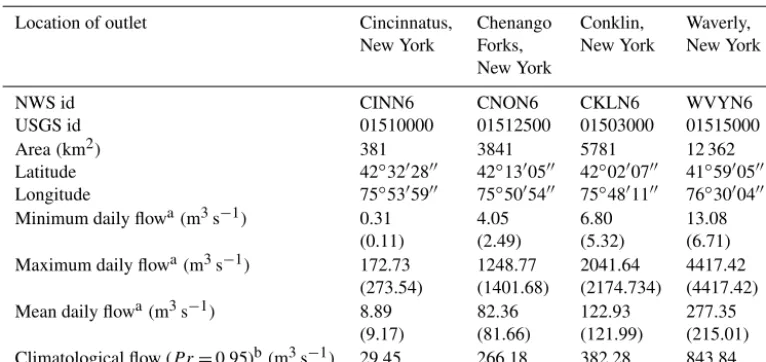
The drainage area of the selected basins ranges from 381 to 12 362 km2. Table 1 outlines some key characteristics of the study basins.

3 Approach

In this section, we describe the different components of the RHEPS, including the hydrometeorological observations, weather forecasts, preprocessor, postprocessors, hydrologi-cal model, and the forecasting experiments and verification strategy.

3.1 Hydrometeorological observations

Three main observation datasets are used: multisensor pre-cipitation estimates (MPEs), gridded near-surface air temper-ature, and daily streamflow. MPEs and gridded near-surface air temperature are used to run the hydrological model in simulation mode for parameter calibration purposes and to initialize the RHEPS. Both the MPEs and gridded near-surface air temperature data at 4×4 km2 resolution were provided by the NOAA’s Middle Atlantic River Forecast Center (MARFC) (Siddique and Mejia, 2017). Similar to the NCEP stage-IV dataset (Moore et al., 2015; Prat and Nelson, 2015), the MARFC’s MPEs represent a continuous time series of hourly, gridded precipitation observations at 4×4 km2 cells, which are produced by combining multi-ple radar estimates and rain gauge measurements. The grid-ded near-surface air temperature data at 4×4 km2resolution were developed by the MARFC by combining multiple tem-perature observation networks as described by Siddique and Mejia (2017). Daily streamflow observations for the selected basins were obtained from the USGS. The streamflow obser-vations are used to verify the simulated flows, and the raw and postprocessed ensemble streamflow forecasts.

3.2 Meteorological forecasts

Table 1.Main characteristics of the four study basins.

Location of outlet Cincinnatus, Chenango Conklin, Waverly, New York Forks, New York New York

New York

NWS id CINN6 CNON6 CKLN6 WVYN6

USGS id 01510000 01512500 01503000 01515000

Area(km2) 381 3841 5781 12 362

Latitude 42◦3202800 42◦1300500 42◦0200700 41◦5900500 Longitude 75◦5305900 75◦5005400 75◦4801100 76◦3000400 Minimum daily flowa(m3s−1) 0.31 4.05 6.80 13.08

(0.11) (2.49) (5.32) (6.71) Maximum daily flowa(m3s−1) 172.73 1248.77 2041.64 4417.42

(273.54) (1401.68) (2174.734) (4417.42) Mean daily flowa(m3s−1) 8.89 82.36 122.93 277.35

(9.17) (81.66) (121.99) (215.01) Climatological flow (P r=0.95)b(m3s−1) 29.45 266.18 382.28 843.84

a_{The numbers in parentheses are the historical (based on entire available record, as opposed to the period 2004–2012 used in this}

study) daily minimum, maximum, or mean recorded flow.bP r=0.95 indicates flows with exceedance probability of 0.05.

the same atmospheric model and initial conditions as the ver-sion 9.0.1 of the Global Ensemble Forecast System and runs at T254L42 (∼0.50◦Gaussian grid spacing or∼55 km) and T190L42 (∼0.67◦Gaussian grid spacing or∼73 km) reso-lutions for the first and second 8 days, respectively (Hamill et al., 2013). The reforecasts are initiated once daily at 00:00 Coordinated Universal Time. Each forecast cycle consists of 3-hourly accumulations for day 1 to day 3 and 6-hourly accu-mulations for day 4 to day 16. In this study, we use 9 years of GEFSRv2 data, from 2004 to 2012, and forecast lead times from 1 to 7 days. The period 2004 to 2012 is selected to take advantage of data that were previously available to us (i.e., GEFSRv2 and MPEs for the MAR) from a recent veri-fication study (Siddique et al., 2015). Forecast lead times of up to 7 days are chosen since we previously found that the GEFSRv2 skill is low after 7 days (Siddique et al., 2015; Sharma et al., 2017). The GEFSRv2 data are bilinearly in-terpolated onto the 4×4 km2grid cell resolution of the HL-RDHM model.

3.3 Distributed hydrological model

NOAA’s HL-RDHM is used as the spatially distributed hy-drological model (Koren et al., 2004). Within HL-RDHM, the Sacramento Soil Moisture Accounting model with Heat Transfer (SAC-HT) is used to represent hillslope runoff gen-eration, and the SNOW-17 module is used to represent snow accumulation and melting.

HL-RDHM is a spatially distributed conceptual model, where the basin system is divided into regularly spaced, square grid cells to account for spatial heterogeneity. Each grid cell acts as a hillslope capable of generating surface, in-terflow, and groundwater runoff that discharges directly into the streams. The cells are connected to each other through

the stream network system. Further, the SNOW-17 module allows each cell to accumulate snow and generate hillslope snowmelt based on the near-surface air temperature. The hill-slope runoff, generated at each grid cell by SAC-HT and SNOW-17, is routed to the stream network using a nonlin-ear kinematic wave algorithm (Koren et al., 2004; Smith et al., 2012a). Likewise, flows in the stream network are routed downstream using a nonlinear kinematic wave algorithm that accounts for parameterized stream cross-section shapes (Ko-ren et al., 2004; Smith et al., 2012a). In this study, we run HL-RDHM using a 2 km horizontal resolution. Further infor-mation about the HL-RDHM can be found elsewhere (Koren et al., 2004; Reed et al., 2007; Smith et al., 2012a; Fares et al., 2014; Rafieeinasab et al., 2015; Thorstensen et al., 2016; Siddique and Mejia, 2017).

OF= v u u t

m X

i=1

qi−si() 2

, (1)

where qi and si denote the daily observed and simulated flows at timei, respectively;is the parameter vector being estimated; and mis the total number of days used for cali-bration. A total of 3 years (2003–2005) of streamflow data are used to calibrate the HL-RDHM for the selected basins. The first year (year 2003) is used to warm up HL-RDHM. To assess the model performance during calibration, we use the percent bias (PB), modified correlation coefficient (Rm), and

Nash–Sutcliffe efficiency (NSE) (see Appendix for details). Note that these metrics are used during the manual phase of the calibration process, and to assess the final results from the implementation of the SLS. However, the actual imple-mentation of the SLS is based on the objective function in Eq. (1).

3.4 Statistical weather preprocessor

Heteroscedastic censored logistic regression (Messner et al., 2014a; Yang et al., 2017) is implemented to preprocess the ensemble precipitation forecasts from the GEFSRv2. HCLR is selected since it offers the advantage, over other regression-based preprocessors (Wilks, 2009), of obtain-ing the full, continuous predictive probability density func-tion (pdf) of precipitafunc-tion forecasts (Messner et al., 2014b). Also, HCLR has been shown to outperform other widely used preprocessors, such as Bayesian model averaging (Yang et al., 2017). In principle, HCLR fits the conditional logis-tic probability distribution function to the transformed (here the square root) ensemble mean and bias corrected precipita-tion ensembles. Note that we tried different transformaprecipita-tions (square root, cube root, and fourth root) and found a similar performance between the square and cube root, both outper-forming the fourth root. In addition, HCLR uses the ensem-ble spread as a predictor, which allows the use of uncertainty information contained in the ensembles.

The development of the HCLR follows the logistic re-gression model initially proposed by Hamill et al. (2004) as well as the extended version of that model proposed by Wilks (2009). The extended logistic regression of Wilks (2009) is used to model the probability of binary re-sponses such that

P (y≤z|x)=3[ω(z)−δ(x)], (2)

where 3(.) denotes the cumulative distribution function of the standard logistic distribution, y is the transformed pre-cipitation, zis a specified threshold, x is a predictor vari-able that depends on the forecast members, δ(x) is a lin-ear function of the predictor variablex, and the transforma-tionω(.) is a monotone nondecreasing function. Messner et al. (2014a) proposed the heteroscedastic extended logistic re-gression (HELR) preprocessor with an additional predictor

variableϕto control the dispersion of the logistic predictive distribution,

P (y≤z|x)=3

_{ω(z)−δ(x)}

exp[η(ϕ)]

, (3)

whereη(.) is a linear function of ϕ. The functionsδ(.) and

η(.) are defined as follows:

δ(x)=a0+a1x (4)

and

η(ϕ)=b0+b1ϕ, (5)

wherea0,a1,b0, andb1are parameters that need to be

esti-mated;x= 1 K

K P

k=1 f

1 2

k , i.e., the predictor variablexis the mean of the transformed, via the square root, ensemble forecastsf;

K is the total number of ensemble members; and ϕ is the standard deviation of the square-root-transformed precipita-tion ensemble forecasts.

Maximum likelihood estimation with the log-likelihood function is used to estimate the parameters associated with Eq. (3) (Messner et al., 2014a, b). One variation of the HELR preprocessor that can easily accommodate nonnegative vari-ables, such as precipitation amounts, is HCLR. For this, the predicted probability or likelihoodπiof theith observed out-come is determined as follows (Messner et al., 2014b):

πi=    

  

3

ω(0)−δ(x)

exp[η(ϕ)]

yi=0

λ _{ω (y}

i)−δ(x) exp[η(ϕ)]

yi>0

, (6)

whereλ[.] denotes the likelihood function of the standard lo-gistic function. As indicated by Eq. (6), HCLR fits a lolo-gistic error distribution with point mass at zero to the transformed predictand.

(Yang et al., 2017). To make the implementation of HCLR as straightforward as possible, the stationary window is used here. Finally, the Schaake shuffle method as applied by Clark et al. (2004) is implemented to maintain the observed space– time variability in the preprocessed GEFSRv2 precipitation forecasts. At each individual forecast time, the Schaake shuf-fle is applied to produce a spatial and temporal rank structure for the ensemble precipitation values that is consistent with the ranks of the observations.

3.5 Statistical streamflow postprocessors

To statistically postprocess the flow forecasts generated by the RHEPS, two different approaches are tested, namely a first-order autoregressive model with a single exogenous variable, ARX(1,1), and quantile regression (QR). We se-lect the ARX(1,1) postprocessor since it has been suggested and implemented for operational applications in the US (Re-gonda et al., 2013). QR is chosen because it is of similar com-plexity to the ARX(1,1) postprocessor but for some forecast-ing conditions it has been shown to outperform it (Mendoza et al., 2016). Furthermore, the ARX (1,1) and QR postpro-cessors have not been compared against each other for the forecasting conditions specified by the RHEPS. The post-processors are implemented for the years 2004–2012, using the same leave-one-out approach used for the preprocessor. For this, the 6-hourly precipitation accumulations are used to force the HL-RDHM and generate 6-hourly flows. Note that we use 6-hourly accumulations since this is the resolution of the GEFSRv2 data after day 4 and this is a temporal reso-lution often used in operational forecasting in the US. Since the observed flow data are mean daily, we compute the mean daily flow forecast from the 6-hourly flows. The postproces-sor is then applied to the mean daily values from day 1 to 7. 3.5.1 First-order autoregressive model with a single

exogenous variable

To implement the ARX(1,1) postprocessor, the observation and forecast data are first transformed into standard nor-mal deviates using the nornor-mal quantile transformation (NQT) (Krzysztofowicz, 1997; Bogner et al., 2012). The trans-formed observations and forecasts are then used as predictors in the ARX(1,1) model (Siddique and Mejia, 2017). Specif-ically, for each forecast lead time, the ARX(1,1) postproces-sor is formulated as follows:

q_iT+1=(1−ci+1) qiT +ci+1fiT+1+ξi+1, (7)

whereq_iT andq_iT₊₁are the NQT-transformed observed flows at time stepsiandi+1, respectively;cis the regression co-efficient;f_iT₊₁is the NQT transformed forecast flow at time stepi+1; andξ is the residual error term. In Eq. (7), assum-ing that there is significant correlation betweenξi+1andqiT,

ξi+1can be calculated as follows:

ξi+1= σξi+1

σξi

ρ (ξi+1, ξi) ξi+ϑi+1, (8)

whereσξiandσξi+1 are the standard deviation ofξiandξi+1,

respectively;ρ(ξi+1,ξi)is the serial correlation betweenξi+1

andξi; andϑi+1is a random Gaussian error generated from N(0,σ_ϑ2

i+1). To estimateN(0,σ 2

ϑi+1), the following equation

is used:

σ_ϑ2 i+1=

h

1−ρ2(ξi+1, ξi) i

σ_ξ2

i+1. (9)

To implement Eq. (7), 10 equally spaced values ofci+1are

selected from 0.1 to 0.9. For each value of ci+1, σ_ϑ2_i+1 is

determined from Eq. (9), using the training data to deter-mine the other variables in Eq. (9). Then,ϑi+1is generated

fromN(0, σ_ϑ2

i+1)andξi+1 is calculated from Eq. (8). The

result from Eq. (8) is used with Eq. (7) to generate a trace of q_iT₊₁ which is transformed back to real space using the inverse NQT. These steps are repeated to generate multiple traces for each value of ci+1. For each value of ci+1, the

ARX(1,1) model is trained and used to generate ensemble streamflow forecasts, which are in turn used to compute the mean continuous ranked probability score (CRPS) for the 7-year training period under consideration. Thus, the mean CRPS is computed for each value of ci+1, and the value

of ci+1 that produces the smallest mean CRPS is then

se-lected for use in the 2-year verification period under consid-eration. This is repeated until all the years (2004–2012) have been postprocessed and verified independently of the training period. The ARX(1,1) postprocessor is applied at each indi-vidual lead time. Thus, at each forecast lead time, an optimal value ofci+1is estimated by minimizing the mean CRPS

fol-lowing the steps previously outlined. For lead times beyond the initial one (day 1), 1-day-ahead predictions are used as the observed streamflow. For the cases in whichq_iT₊₁ falls beyond the historical maxima, extrapolation is used by mod-eling the upper tail of the forecast distribution as hyperbolic (Journel and Huijbregts, 1978).

3.5.2 Quantile regression

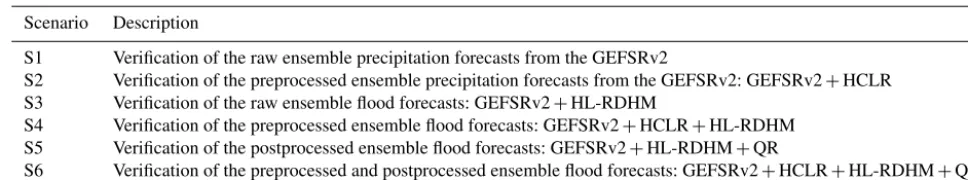
Table 2.Summary and description of the verification scenarios.

Scenario Description

S1 Verification of the raw ensemble precipitation forecasts from the GEFSRv2

S2 Verification of the preprocessed ensemble precipitation forecasts from the GEFSRv2: GEFSRv2+HCLR S3 Verification of the raw ensemble flood forecasts: GEFSRv2+HL-RDHM

S4 Verification of the preprocessed ensemble flood forecasts: GEFSRv2+HCLR+HL-RDHM S5 Verification of the postprocessed ensemble flood forecasts: GEFSRv2+HL-RDHM+QR

S6 Verification of the preprocessed and postprocessed ensemble flood forecasts: GEFSRv2+HCLR+HL-RDHM+QR

lead time, the mathematical notation does not reflect this for simplicity.

The QR model is given by

ε_τ0 =dτ+eτf , (10)

whereε0_τ is the error estimate at quantile intervalτ,f is the ensemble mean, anddτ andeτ are the linear regression co-efficients aτ. The coefficients are determined by minimizing the sum of the residuals based on the training data as follows:

min N X

i=1

wτετ,i−ετ0 i, fi

. (11)

Here, ετ,i and fi are the paired samples from a total of

N samples;ετ,i is computed as the observed flow minus the forecasted one,qτ−fτ; andwτ is the weighting function for theτth quantile defined as follows:

wτ(ζi)=

(τ−1)ζi ifζi≤0

τ ζi ifζi>0

, (12)

where ζi is the residual term defined as the difference be-tweenετ,i andετ0(i,fi)for the quantile τ. The minimiza-tion in Eq. (11) is solved using linear programming (Koenker, 2005).

Lastly, to obtain the calibrated forecast,fτ, the following equation is used:

fτ =f+ε0τ. (13)

In Eq. (13), the estimated error quantiles and the ensemble mean are added to form a calibrated discrete quantile rela-tionship for a particular forecast lead time and thus generate an ensemble streamflow forecast.

3.6 Forecast experiments and verification

The verification analysis is carried out using the Ensemble Verification System (Brown et al., 2010). For the verification, the following metrics are considered: Brier skill score (BSS), mean continuous ranked probability skill score (CRPSS), and the decomposed components of the CRPS (Hersbach, 2000), i.e., the CRPS reliability (CRPSrel) and CRPS

po-tential (CRPSpot). The definition of each of these metrics is

provided in the appendix. Additional details about the verifi-cation metrics can be found elsewhere (Wilks, 2011; Jolliffe and Stephenson, 2012). Confidence intervals for the verifica-tion metrics are determined using the staverifica-tionary block boot-strap technique (Politis and Romano, 1994), as done by Sid-dique et al. (2015). All the forecast verifications are done for lead times from 1 to 7 days.

To verify the forecasts for the period 2004–2012, six dif-ferent forecasting scenarios are considered (Table 2). The first (S1) and second (S2) scenario verify the raw and prepro-cessed ensemble precipitation forecasts, respectively. Sce-narios 3 (S3), 4 (S4), and 5 (S5) verify the raw, prepro-cessed, and postprocessed ensemble streamflow forecasts, re-spectively. The last scenario, S6, verifies the combined pre-processed and postpre-processed ensemble streamflow forecasts. In S1 and S2, the raw and preprocessed ensemble precipita-tion forecasts are verified against the MPEs. For the verifica-tion of S1 and S2, each grid cell is treated as a separate veri-fication unit. Thus, for a particular basin, the average perfor-mance is obtained by averaging the verification results from different verification units. The streamflow forecast scenar-ios, S3–S6, are verified against mean daily streamflow ob-servations from the USGS. The quality of the streamflow forecasts is evaluated conditionally upon forecast lead time, season (cool and warm), and flow threshold.

4 Results and discussion

This section is divided into four subsections. The first subsec-tion demonstrates the performance of the spatially distributed model, HL-RDHM. The second subsection describes the per-formance of the raw and preprocessed GEFSRv2 ensemble precipitation forecasts (forecasting scenarios S1 and S2). In the third subsection, the two statistical postprocessing tech-niques are compared. Lastly, the verification of different ensemble streamflow forecasting scenarios is shown in the fourth subsection (forecasting scenarios S3–S6).

(a)

Rm

0 0.2 0.4 0.6 0.8 1

(b)

NSE

0 0.2 0.4 0.6 0.8 1

(c)

PB

−20 −15 −10 −5 0 5 10

Uncalibrated Calibrated CINN6 CNON6 CKLN6 WVYN6

CINN6 CNON6 CKLN6 WVYN6 CINN6 CNON6 CKLN6 WVYN6

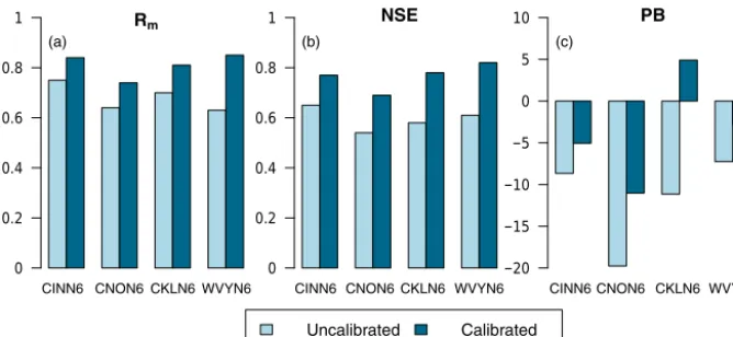
Figure 2.Performance statistics for the uncalibrated and calibrated simulation runs for the entire period of analysis (years 2004–2012):

(a)Rm,(b)NSE, and(c)PB.

(years 2004–2012). Note that the simulated flows are ob-tained by forcing HL-RDHM with gridded observed precip-itation and near-surface temperature data. The verification is done for the four basin outlets shown in Fig. 1. To perform the verification and assess the quality of the streamflow simu-lations, the following statistical measures of performance are employed: modified correlation coefficient, Nash–Sutcliffe efficiency, and percent bias. The mathematical definition of these metrics is provided in the appendix. The verification is done for both uncalibrated and calibrated simulation runs for the entire period of analysis. The main results from the verification of the streamflow simulations are summarized in Fig. 2.

The performance of the calibrated simulation runs is satisfactory, with Rm values ranging from ∼0.75 to 0.85

(Fig. 2a). Likewise, the NSE, which is sensitive to both the correlation and bias, ranges from∼0.69 to 0.82 for the cali-brated runs (Fig. 2b), while the PB ranges from∼5 to−11 % (Fig. 2c). Relative to the uncalibrated runs, theRm, NSE, and

PB values improve by∼18, 29, and 47 %, respectively. Fur-ther, the performance of the calibrated simulation runs is sim-ilar across the four selected basins, although the largest basin, WVYN6 (Fig. 2), shows slightly higher performance with

Rm, NSE, and PB values of 0.85, 0.82, and−3 % (Fig. 2),

re-spectively. The lowest performance is seen in CNON6 with

Rm, NSE, and PB values of 0.75, 0.7, and−11 % (Fig. 2),

respectively. Nonetheless, the performance metrics for both the uncalibrated and calibrated simulation runs do not deviate widely from each other in the selected basins, with perhaps the only exception being PB (Fig. 2c).

4.2 Verification of the raw and preprocessed ensemble precipitation forecasts

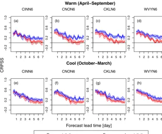
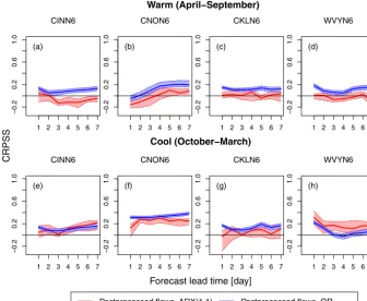
To examine the skill of both the raw and preprocessed GEF-SRv2 ensemble precipitation forecasts, we plot in Fig. 3 the CRPSS (relative to sampled climatology) as a function of the

forecast lead time (day 1 to 7) and season for the selected basins. Two seasons are considered: cool (October–March) and warm (April–September). Note that a CRPSS value of zero means no skill (i.e., same skill as the reference system) and a value of 1 indicates maximum skill. The CRPSS is computed using 6-hourly precipitation accumulations.

The skill of both the raw and preprocessed ensemble pre-cipitation forecasts tends to decline with increasing fore-cast lead time (Fig. 3). In the warm season (Fig. 3a–d), the CRPSS values vary overall, across all the basins, in the range from∼0.17 to 0.5 and from∼0.0 to 0.4 for the pre-processed and raw forecasts, respectively; while in the cool season (Fig. 3e–h) the CRPSS values vary overall in the range from∼0.2 to 0.6 and from ∼0.1 to 0.6 for the pre-processed and raw forecasts, respectively. The skill of the preprocessed ensemble precipitation forecasts tends to be greater than the raw ones across basins, seasons, and forecast lead times. Comparing the raw and preprocessed forecasts against each other, the relative skill gains from preprocess-ing are somewhat more apparent in the medium-range lead times (>3 days) and warm season. That is, the differences in skill seem not as significant in the short-range lead times (≤3 days). This seems particularly the case in the cool sea-son, where the confidence intervals for the raw and prepro-cessed forecasts tend to overlap (Fig. 3e–h).

CINN6

1 2 3 4 5 6 7

−0.2

0.2

0.6

1.0

(a)

CNON6

1 2 3 4 5 6 7

−0.2

0.2

0.6

1.0

(b)

CKLN6

1 2 3 4 5 6 7

−0.2

0.2

0.6

1.0

(c)

WVYN6

1 2 3 4 5 6 7

−0.2

0.2

0.6

1.0

(d)

CINN6

1 2 3 4 5 6 7

−0.2

0.2

0.6

1.0

(e)

CNON6

1 2 3 4 5 6 7

−0.2

0.2

0.6

1.0

(f)

CKLN6

1 2 3 4 5 6 7

−0.2

0.2

0.6

1.0

(g)

WVYN6

1 2 3 4 5 6 7

−0.2

0.2

0.6

1.0

(h)

Raw precipitation Preprocessed precipitation

CRPSS

Forecast lead time [day]

Warm (April−September)

Cool (October−March)

Figure 3.CRPSS (relative to sampled climatology) of the raw (red curves) and preprocessed (blue curves) ensemble precipitation forecasts

from the GEFSRv2 vs. the forecast lead time during the(a)–(d)warm (April–September) and(e)–(h)cool season (October–March) for the selected basins.

basins tend to display similar performance; i.e. the analysis does not reflect skill sensitivity to the basin size as in other studies (Siddique et al., 2015; Sharma et al., 2017). This is expected here since the verification is performed for each GEFSRv2 grid cell, rather than verifying the average for the entire basin. That is, the results in Fig. 3 are for the aver-age skill performance obtained from verifying each individ-ual grid cell within the selected basins.

Based on the results presented in Fig. 3, we may expect some skill contribution to the streamflow ensembles from forcing the HL-RDHM with the preprocessed precipitation, as opposed to using the raw forecast forcing. It may also be expected that the contributions are greater for the medium-range lead times and warm season. This will be examined in Sect. 4.4; prior to that we compare next the two postproces-sors, namely ARX(1,1) and QR.

4.3 Selection of the streamflow postprocessor

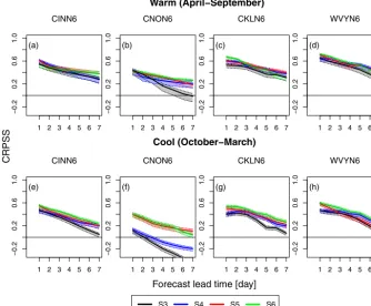
The ability of the ARX(1,1) and QR postprocessors to im-prove ensemble streamflow forecasts is investigated here. The postprocessors are applied to the raw streamflow ensem-bles at each forecast lead time from day 1 to 7. To examine the skill of the postprocessed streamflow forecasts, Fig. 4 dis-plays the CRPSS (relative to the raw ensemble streamflow forecasts) versus the forecast lead time for all the selected

basins, for both warm (Fig. 4a–d) and cool (Fig. 4e–h) sea-sons. In the cool season (Fig. 4e–h), the tendency is for both postprocessing techniques to demonstrate improved forecast skill across all the basins and lead times. The skill can im-prove as much as 40 % at the later lead times (Fig. 4f). The skill improvements, however, from the ARX(1,1) postpro-cessor are not as consistent for the warm season (Fig. 4a–d), displaying negative skill values for some of the lead times in all the basins. The latter underscores an inability of the ARX(1,1) postprocessor to enhance the raw streamflow en-sembles for the warm season. In some cases (Fig. 4b and e–f), the skill of the postprocessors shows an increasing trend with the lead time. This is the case since the skill is here measured relative to the raw streamflow forecasts, which is done to bet-ter isolate the effect of the postprocessors on the streamflow forecasts.

CINN6

1 2 3 4 5 6 7

−0.2

0.2

0.6

1.0

(a)

CNON6

1 2 3 4 5 6 7

−0.2

0.2

0.6

1.0

(b)

CKLN6

1 2 3 4 5 6 7

−0.2

0.2

0.6

1.0

(c)

WVYN6

1 2 3 4 5 6 7

−0.2

0.2

0.6

1.0

(d)

CINN6

1 2 3 4 5 6 7

−0.2

0.2

0.6

1.0

(e)

CNON6

1 2 3 4 5 6 7

−0.2

0.2

0.6

1.0

(f)

CKLN6

1 2 3 4 5 6 7

−0.2

0.2

0.6

1.0

(g)

WVYN6

1 2 3 4 5 6 7

−0.2

0.2

0.6

1.0

(h)

Postprocessed flows, ARX(1,1) Postprocessed flows, QR

CRPSS

Forecast lead time [day]

Warm (April−September)

Cool (October−March)

Figure 4.CRPSS (relative to the raw forecasts) of the ARX(1,1) (red curves) and QR (blue curves) postprocessed ensemble flood forecasts

vs. the forecast lead time during the(a)–(d)warm (April–September) and(e)–(h)cool season (October–March) for the selected basins.

Fig. 4h, but in the warm season QR tends to consistently perform better than ARX(1,1). The overall trend in Fig. 4 is for QR to mostly outperform ARX(1,1), with the differ-ence in performance being as high as 30 % (Fig. 4d at the day 7 lead time). This is noticeable across all the basins (ex-cept WVYN6 in Fig. 4h) for most of the lead times and for both seasons.

As discussed and demonstrated in Fig. 4, QR performs bet-ter than ARX(1,1). We also computed reliability diagrams, as determined by Sharma et al. (2017), for the two postproces-sors (plots not shown) and found that QR tends to display bet-ter reliability than ARX(1,1) across lead times, basins, and seasons. Therefore, we select QR as the statistical streamflow postprocessor to examine the interplay between preprocess-ing and postprocesspreprocess-ing in the RHEPS.

4.4 Verification of the ensemble streamflow forecasts for different statistical processing scenarios

In this subsection, we examine the effects of different statis-tical processing scenarios on the ensemble streamflow fore-casts from the RHEPS. The forecasting scenarios considered here are S3–S6 (Table 2 defines the scenarios). To facilitate presenting the verification results, this subsection is divided into the following three parts: CRPSS, CRPS decomposition, and BSS.

4.4.1 CRPSS

The skill of the ensemble streamflow forecasts for S3–S6 is assessed using the CRPSS relative to the sampled climatol-ogy (Fig. 5). The CRPSS in Fig. 5 is shown as a function of the forecast lead time for all the basins, and the warm (Fig. 5a–d) and cool (Fig. 5e–h) seasons. The most salient feature of Fig. 5 is that the performance of the streamflow forecasts tends for the most part to progressively improve from S3 to S6. This means that the forecast skill tends to improve across lead times, basin sizes, and seasons as addi-tional statistical processing steps are included in the RHEPS forecasting chain. Although there is some tendency for the large basins to show better forecast skill than the small ones, the scaling (i.e., the dependence of skill on the basin size) is rather mild and not consistent across the four basins.

CINN6

1 2 3 4 5 6 7

−0.2

0.2

0.6

1.0

(a)

CNON6

1 2 3 4 5 6 7

−0.2

0.2

0.6

1.0

(b)

CKLN6

1 2 3 4 5 6 7

−0.2

0.2

0.6

1.0

(c)

WVYN6

1 2 3 4 5 6 7

−0.2

0.2

0.6

1.0

(d)

CINN6

1 2 3 4 5 6 7

−0.2

0.2

0.6

1.0

(e)

CNON6

1 2 3 4 5 6 7

−0.2

0.2

0.6

1.0

(f)

CKLN6

1 2 3 4 5 6 7

−0.2

0.2

0.6

1.0

(g)

WVYN6

1 2 3 4 5 6 7

−0.2

0.2

0.6

1.0

(h)

S3 S4 S5 S6

CRPSS

Forecast lead time [day]

Warm (April−September)

Cool (October−March)

Figure 5. Continuous ranked probability skill score (CRPSS) of the mean ensemble flood forecasts vs. the forecast lead time during the

(a)–(d)warm (April–September) and(e)–(h)cool season (October–March) for the selected basins. The curves represent the different fore-casting scenarios S3–S6. Note that S3 consists of GEFSRv2+HL-RDHM, S4 of GEFSRv2+HCLR+HL-RDHM, S5 of GEFSRv2+ HL-RDHM+QR, and S6 of GEFSRv2+HCLR+HL-RDHM+QR.

then shows further improvements for both S5 and S6, rela-tive to S4. Although S6 tends to outperform both S4 and S5 in Fig. 5, the differences in skill among these three scenar-ios are not as significant; their confidence intervals tend to overlap in most cases, with the exception of Fig. 5f, in which S4 underperforms relative to both S5 and S6. Figure 5 shows that S6 is the preferred scenario in that it tends to more con-sistently improve the ensemble streamflow forecasts across basins, lead times, and seasons than the other scenarios. It also shows that postprocessing alone, S5, may be slightly more effective than preprocessing alone, S4, in correcting the streamflow forecast biases.

There are also seasonal differences in the forecast skill among the scenarios. The skill of the streamflow forecasts tends to be slightly greater in the warm season (Fig. 5a–d) than in the cool one (Fig. 5e–h) across all the basins and lead times. In the warm season (Fig. 5a–d), all the scenarios tend to show similar skill, except CNON6 (Fig. 5b), with S5 and S6 only slightly outperforming S3 and S4. In the cool sea-son (Fig. 5e–h), with the exception of CNON6 (Fig. 5f), the performance is similar among the scenarios for the short lead times, but S3 tends to consistently underperform for the later lead times relative to S4–S6. There is also a skill reversal between the seasons when comparing the ensemble precipi-tation (Fig. 3) and streamflow (Fig. 5) forecasts. That is, the

skill tends to be higher in the cool season than the warm one in Fig. 3, but this trend reverses in Fig. 5. The reason for this reversal is that in the cool season hydrological conditions are strongly influenced by snow dynamics, which can be chal-lenging to represent with HL-RDHM, particularly when spe-cific snow information or data are not available. In any case, this could be a valuable area for future research since it ap-pears here to have a significant influence on the skill of the ensemble streamflow forecasts.

(a)

0 2 4 6

S3 S4 S5

S6

Warm (April−September) CINN6

(e)

Cool (October−March) CINN6

0 2 4 6

(b)

CNON6

0 25 50 75

(f)

CNON6

0 25 50 75

(c)

CKLN6

0 25 50 75

(g)

CKLN6

0 25 50 75

(d)

WVYN6

0 25 50 75 100 125

(h)

WVYN6

0 25 50 75 100 125

Day1 Day3 Day7

Day1 Day3 Day7

CRPSpot CRPSrel

C

R

P

S

(

m

s

3

−

1

)

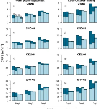
Figure 6.Decomposition of the CRPS into CRPS potential (CRPSpot) and CRPS reliability (CRPSrel) for forecasts lead times of 1, 3, and

7 days during the warm(a)–(d)(April–September) and cool season(e)–(h)(October–March) for the selected basins. The four columns asso-ciated with each forecast lead time represent the forecasting scenarios S3–S6 (from left to right). Note that S3 consists of GEFSRv2+ HL-RDHM, S4 of GEFSRv2+HCLR+HL-RDHM, S5 of GEFSRv2+HL-RDHM+QR, and S6 of GEFSRv2+HCLR+HL-RDHM+QR.

in Fig. 2c), where the performance of CNON6 is somewhat lower than in the other basins. Interestingly, after postpro-cessing (S5 in Fig. 5f), the skill of CNON6 is as good as that of CINN6, even though at the day 1 lead time the skill for S3 is ∼0.1 for CNON6 (Fig. 5f) and∼0.4 for CINN6 (Fig. 5e). Hence, the postprocessor seems capable of com-pensating somewhat for the lesser performance of CNON6 in both calibration or after preprocessing in the cool season. 4.4.2 CRPS decomposition

Figure 6 displays different components of the mean CRPS against lead times of 1, 3, and 7 days for all the basins ac-cording to both the warm (Fig. 6a–d) and cool (Fig. 6e– h) seasons. The components presented here are reliabil-ity (CRPSrel) and potential CRPS (CRPSpot) (Hersbach,

2000). CRPSrel measures the average reliability of the

en-semble forecasts across all the possible events, i.e., it exam-ines whether the fraction of observations that fall below the

jth ofnranked ensemble members is equal toj/non aver-age. CRPSpotrepresents the lowest possible CRPS that could

be obtained if the forecasts were made perfectly reliable (i.e., CRPSrel=0). Note that the CRPS, CRPSrel, and CRPSpotare

all negatively oriented, with perfect score of zero. Overall, as was the case with the CRPSS (Fig. 5), the CRPS decomposi-tion reveals that forecast reliability tends mostly to progres-sively improve from S3 to S6.

Interestingly, improvements in forecast quality for S5 and S6, relative to the raw streamflow forecasts of S3, are mainly due to reductions in CRPSrel (i.e., by making the

CINN6

0.95 0.97 0.99

0

0.2

0.6

1.0

(a)

CNON6

0.95 0.97 0.99

0

0.2

0.6

1.0

(b)

CKLN6

0.95 0.97 0.99

0

0.2

0.6

1.0

(c)

WVYN6

0.95 0.97 0.99

0

0.2

0.6

1.0

(d)

CINN6

0.95 0.97 0.99

0

0.2

0.6

1.0

(e)

CNON6

0.95 0.97 0.99

0

0.2

0.6

1.0

(f)

CKLN6

0.95 0.97 0.99

0

0.2

0.6

1.0

(g)

WVYN6

0.95 0.97 0.99

0

0.2

0.6

1.0

(h)

Day1 Day1

Day3 Day3

Day7 (obs) Day7 (sim)

Br

ier skill score

Non−exceedance probability

S5 (Warm season)

S6 (Warm season)

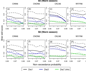
Figure 7.Brier skill score (BSS) of the mean ensemble flood forecasts for S5(a–d)and S6(e–h)vs. the flood threshold for forecast lead

times of 1, 3, and 7 days during the warm (April–September) season for the selected basins. The BSS is shown relative to both observed (solid lines) and simulated floods (dashed lines).

CRPSpotappears to play a bigger role in S4 than in the other

scenarios, since in many cases in Fig. 6 the CRPSpotvalue

for S4 is the lowest among all the scenarios. The explanation for this lies in the implementation of the HCLR preproces-sor, which uses the ensemble spread as a predictor of the dispersion of the predictive pdf and the CRPSpot is

sensi-tive to the spread (Messner et al., 2014a). In terms of the warm and cool seasons, the warm season tends to show a slightly lower CRPS than the cool one for all the scenar-ios. There are other, more nuanced differences between the two seasons. For example, S5 is more reliable than S4 in several cases in Fig. 6, such as for the day 1 lead time in the cool season. The CRPS decomposition demonstrates that the ensemble streamflow forecasts for S5 and S6 tend to be more reliable than for S3 and S4. It also shows that the fore-casts from S5 and S6 tend to exhibit comparable reliability. However, the ensemble streamflow forecasts generated using both preprocessing and postprocessing, S6, ultimately result in lower CRPS than the other scenarios. The latter is seen across all the basins, lead times, and seasons, except in one case (Fig. 6d at the day 7 lead time).

4.4.3 BSS

In our final verification comparison, the BSS values of the ensemble streamflow forecasts for S5 (Fig. 7a–d) and S6 (Fig. 7e–h) are plotted against the non-exceedance proba-bility associated with different streamflow thresholds ranging from 0.95 to 0.99. The BSS is computed for all the basins, for the warm season, and at lead times of 1, 3 and 7 days. In addition, the BSS is computed relative to both observed (solid lines in Fig. 7) and simulated (dashed lines in Fig. 7) flows. When the BSS is computed relative to observed flows, it considers the effect on forecast skill of both meteorologi-cal and hydrologimeteorologi-cal uncertainties. While the BSS relative to simulated flows is mainly affected by meteorological uncer-tainties. The difference between the two, i.e., the BSS rela-tive to observed flows minus the BSS relarela-tive to simulated ones, provides an estimate of the effect of hydrological un-certainties on the skill of the streamflow forecasts. Similar to the CRPSS, the BSS value of zero means no skill (i.e., same skill as the reference system) and a value of 1 indicates per-fect skill.

the different flow thresholds appear similar for S5 (Fig. 7a– d) and S6 (Fig. 7e–h). The only exception is CKLN6 (Fig. 7c and g), where S6 has better skill than S5 at the day 1 and 3 lead times, particularly at the highest flow thresholds consid-ered. With respect to the basin size, the skill tends to improve somewhat from the small to the large basin. For instance, for non-exceedance probabilities of 0.95 and 0.99 at the day 1 lead time, the BSS values for the smallest basin (Fig. 7a), measured relative to the observed flows, are∼0.49 and 0.35, respectively. For the same conditions, both values increase to∼0.65 for the largest basin (Fig. 7d).

The most notable feature in Fig. 7 is that the effect of hydrological uncertainties on forecast skill is evident at the day 1 lead time, while meteorological uncertainties clearly dominate at the day 7 lead time. With respect to the latter, notice that the solid and dashed green lines for the day 7 lead time tend to be very close to each other in Fig. 7, indicat-ing that hydrological uncertainties are relatively small com-pared to meteorological ones. Hydrological uncertainties are largest at the day 1 lead time, particularly for the small basins (Fig. 7a–b and e–f). For example, for a non-exceedance prob-ability of 0.95 and at a day 1 lead time (Fig. 7b), the BSS value relative to the simulated and observed flows are∼0.79 and 0.38, respectively, suggesting a reduction of∼50 % skill due to hydrological uncertainties.

5 Summary and conclusion

In this study, we used the RHEPS to investigate the effect of statistical processing on short- to medium-range ensemble streamflow forecasts. First, we assessed the raw precipita-tion forecasts from the GEFSRv2 (S1), and compared them with the preprocessed precipitation ensembles (S2). Then, streamflow ensembles were generated with the RHEPS for four different forecasting scenarios involving no statistical processing (S3), preprocessing alone (S4), postprocessing alone (S5), and both preprocessing and postprocessing (S6). The verification of ensemble precipitation and streamflow forecasts was done for the years 2004–2012, using four nested gauge locations in the NBSR basin of the US MAR. We found that the scenario involving both preprocessing and postprocessing consistently outperforms the other scenarios. In some cases, however, the differences between the scenario involving preprocessing and postprocessing, and the scenario with postprocessing alone are not as significant, suggesting for those cases (e.g., warm season) that postprocessing alone can be effective in removing systematic biases. Other specific findings are as follows:

– The HCLR preprocessed ensemble precipitation fore-casts show improved skill relative to the raw forefore-casts. The improvements are more noticeable in the warm sea-son at the longer lead times (>3 days).

– Both postprocessors, ARX(1,1) and QR, show gains in skill relative to the raw ensemble streamflow forecasts in the cool season. In contrast, in the warm season, ARX(1,1) shows little or no gains in skill. Overall, for the majority of cases analyzed, the gains with QR tend to be greater than with ARX(1,1), especially during the warm season.

– In terms of the forecast skill (i.e., CRPSS), in the warm season the scenarios including only preprocessing and only postprocessing have a comparable performance to the more complex scenario consisting of both prepro-cessing and postproprepro-cessing, while in the cool season, the scenario involving both preprocessing and postpro-cessing consistently outperforms the other scenarios but the differences may not be as significant.

– The skill of the postprocessing-alone scenario and the scenario that combines preprocessing and postprocess-ing was further assessed uspostprocess-ing the Brier skill score for different streamflow thresholds and the warm season. This assessment suggests that for high flow thresholds the similarities in skill between both scenarios, S5 and S6, become greater.

– Decomposing the CRPS into reliability and poten-tial components, we observed that the scenario that combines preprocessing and postprocessing results in slightly lower CRPS than the other scenarios. We found that the scenario involving only postprocessing tends to demonstrate similar reliability to the scenario consisting of both preprocessing and postprocessing across most of the lead times, basins, and seasons. We also found that in several cases the postprocessing-alone scenario dis-plays improved reliability relative to the preprocessing-alone scenario.

These conclusions are specific to the RHEPS forecasting sys-tem, which is mostly relevant to the US research and opera-tional communities as it relies on a weather and a hydrologi-cal model that are used in this domain. However, the use of a global weather forecasting system illustrates the potential of applying the statistical techniques tested here in other regions worldwide.

conditions and hydrological parameters could be performed. For instance, the combined use of data assimilation and post-processing has been shown to produce more reliable and sharper streamflow forecasts (Bourgin et al., 2014). The po-tential for the interaction of preprocessing and postprocess-ing with data assimilation to significantly enhance stream-flow predictions, however, has not been investigated. This could be investigated in the future with the RHEPS, as the pairing of data assimilation with preprocessing and postpro-cessing could facilitate translating the improvements in the preprocessed meteorological forcing down the hydrological forecasting chain.

Appendix A: Verification metrics

Modified correlation coefficient. The modified version of the correlation coefficient, called a modified correlation coeffi-cient Rm, compares event-specific observed and simulated

hydrographs (McCuen and Snyder, 1975). In the modified version, an adjustment factor based on the ratio of the ob-served and simulated flow is introduced to refine the con-ventional correlation coefficientR. The modified correlation coefficientRmis defined as follows:

Rm=R

minσs, σq maxσs, σq

, (A1)

whereσs andσqdenote the standard deviation of the

simu-lated and observed flows, respectively.

Percent bias. PB measures the average tendency of the simulated flows to be larger or smaller than their observed counterparts. Its optimal value is 0.0 where positive values indicate model overestimation bias, and negative values in-dicate model underestimation bias. The PB is estimated as follows:

PB= N P

i=1

(si−qi)

N P

i=1 qi

×100, (A2)

wheresi andqi denote the simulated and observed flow, re-spectively, at timei.

Nash–Sutcliffe efficiency. the NSE (Nash and Sutcliffe, 1970) is defined as the ratio of the residual variance to the initial variance. It is widely used to indicate how well the simulated flows fit the observations. The range of NSE can vary between negative infinity to 1.0, with 1.0 representing the optimal value and values should be larger than 0.0 to in-dicate minimally acceptable performance. The NSE is com-puted as follows:

NSE=1− N P

i=1

(si−qi)2

N P

i=1 qi−qi

2

, (A3)

wheresi,qi, andqi are the simulated, observed, and mean observed flow, respectively, at timei.

Brier skill score. the Brier score (Brier, 1950) is analogous to the mean squared error, but where the forecast is a prob-ability and the observation is either a 0.0 or 1.0. The BS is given by

BS=1 n

n X

i=1

Ffi(z)−Fqi(z) 2

, (A4)

where the probability offi to exceed a fixed thresholdzis

Ffi(z)=Pr

fi> z

. (A5)

Here, n is again the total number of forecast-observation pairs, and

Fqi(z)=

1, qi > z

0, otherwise. (A6)

In order to compare the skill score of the main forecast sys-tem with respect to the reference forecast, it is convenient to define the Brier Skill Score (BSS):

BSS=1− BSmain BSreference

(A7) where BSmainand BSreference are the BS values for the main

forecast system (i.e. the system to be evaluated) and refer-ence forecast system, respectively. Any positive values of the BSS, from 0 to 1, indicate that the main forecast system per-forms better than the reference forecast system. Thus, a BSS of 0 indicates no skill and a BSS of 1 indicates perfect skill.

Mean continuous ranked probability skill score. Continu-ous ranked probability score (CRPS) quantifies the integrated square difference between the cumulative distribution func-tion (cdf) of a forecast,Ff(z), and the corresponding cdf of

the observation,Fq(z). The CRPS is given by

CRPS= ∞ Z

−∞

Ff(z)−Fq(z)2dz. (A8)

To evaluate the skill of the main forecast system relative to the reference forecast system, the associated skill score, the mean continuous ranked probability skill score (CRPSS) is defined as follows:

CRPSS=1− CRPSmain CRPSreference

, (A9)

where the CRPS is averaged across n pairs of forecasts and observations to calculate the mean CRPS of the main forecast system (CRPSmain) and reference forecast

sys-tem (CRPSreference). The CRPSS varies from−∞to 1. Any

positive values of the CRPSS, from 0 to 1, indicate that the main forecast system performs better than the reference fore-cast system.

To further explore the forecast skill, the CRPSmainis

de-composed into the CRPS reliability (CRPSrel) and

poten-tial (CRPSpot) such that CRPSmaincan be calculated as

fol-lows (Hersbach, 2000):

CRPSmain=CRPSrel+CRPSpot. (A10)

The CRPSrelmeasures the average reliability of the

precipita-tion ensembles similarly to the rank histogram, which shows whether the frequency that the verifying analysis was found in a given bin is equal for all bins (Hersbach, 2000). The CRPSpotmeasures the CRPS that one would obtain for a

Competing interests. The authors declare that they have no conflict of interest.

Acknowledgements. We acknowledge the funding support pro-vided by the NOAA/NWS through award NA14NWS4680012.

Edited by: Shraddhanand Shukla

Reviewed by: Michael Scheuerer and two anonymous referees

References

Abaza, M., Anctil, F., Fortin, V., and Perreault, L.: On the incidence of meteorological and hydrological processors: effect of reso-lution, sharpness and reliability of hydrological ensemble fore-casts, J. Hydrol., 555, 371–384, 2017.

Addor, N., Jaun, S., Fundel, F., and Zappa, M.: An operational hydrological ensemble prediction system for the city of Zurich (Switzerland): skill, case studies and scenarios, Hydrol. Earth Syst. Sci., 15, 2327–2347, https://doi.org/10.5194/hess-15-2327-2011, 2011.

Alfieri, L., Burek, P., Dutra, E., Krzeminski, B., Muraro, D., Thie-len, J., and Pappenberger, F.: GloFAS – global ensemble stream-flow forecasting and flood early warning, Hydrol. Earth Syst. Sci., 17, 1161–1175, https://doi.org/10.5194/hess-17-1161-2013, 2013.

Alfieri, L., Pappenberger, F., Wetterhall, F., Haiden, T., Richardson, D., and Salamon, P.: Evaluation of ensemble streamflow predic-tions in Europe, J. Hydrol., 517, 913–922, 2014.

Anderson, R. M., Koren, V. I., and Reed, S. M.: Using SSURGO data to improve Sacramento Model a priori parameter estimates, J. Hydrol., 320, 103–116, 2006.

Baxter, M. A., Lackmann, G. M., Mahoney, K. M., Workoff, T. E., and Hamill, T. M.: Verification of quantitative precipitation re-forecasts over the southeastern United States, Weather Forecast., 29, 1199–1207, 2014.

Bennett, J. C., Robertson, D. E., Shrestha, D. L., Wang, Q., Enever, D., Hapuarachchi, P., and Tuteja, N. K.: A System for Continuous Hydrological Ensemble Forecasting (SCHEF) to lead times of 9days, J. Hydrol., 519, 2832–2846, 2014.

Benninga, H.-J. F., Booij, M. J., Romanowicz, R. J., and Rientjes, T. H. M.: Performance of ensemble streamflow forecasts under var-ied hydrometeorological conditions, Hydrol. Earth Syst. Sci., 21, 5273–5291, https://doi.org/10.5194/hess-21-5273-2017, 2017. Bogner, K., Pappenberger, F., and Cloke, H. L.: Technical Note:

The normal quantile transformation and its application in a flood forecasting system, Hydrol. Earth Syst. Sci., 16, 1085–1094, https://doi.org/10.5194/hess-16-1085-2012, 2012.

Bourgin, F., Ramos, M.-H., Thirel, G., and Andreassian, V.: In-vestigating the interactions between data assimilation and post-processing in hydrological ensemble forecasting, J. Hydrol., 519, 2775–2784, 2014.

Brier, G. W.: Verification of forecasts expressed in terms of proba-bility, Mon. Weather Rev., 78, 1–3, 1950.

Brown, J. D. and Seo, D.-J.: A nonparametric postprocessor for bias correction of hydrometeorological and hydrologic ensemble forecasts, J. Hydrometeorol., 11, 642–665, 2010.

Brown, J. D., Demargne, J., Seo, D.-J., and Liu, Y.: The Ensemble Verification System (EVS): A software tool for verifying ensem-ble forecasts of hydrometeorological and hydrologic variaensem-bles at discrete locations, Environ. Model. Softw., 25, 854–872, 2010. Brown, J. D., He, M., Regonda, S., Wu, L., Lee, H., and Seo, D.-J.:

Verification of temperature, precipitation, and streamflow fore-casts from the NOAA/NWS Hydrologic Ensemble Forecast Ser-vice (HEFS): 2. Streamflow verification, J. Hydrol., 519, 2847– 2868, 2014.

Clark, M., Gangopadhyay, S., Hay, L., Rajagopalan, B., and Wilby, R.: The Schaake shuffle: A method for reconstructing space–time variability in forecasted precipitation and temperature fields, J. Hydrometeorol., 5, 243–262, 2004.

Cloke, H. and Pappenberger, F.: Ensemble flood forecasting: a re-view, J. Hydrol., 375, 613–626, 2009.

Dankers, R., Arnell, N. W., Clark, D. B., Falloon, P. D., Fekete, B. M., Gosling, S. N., Heinke, J., Kim, H., Masaki, Y., Satoh, Y., Stacke, T., Wada, Y., and Wisser, D.: First look at changes in flood hazard in the Inter-Sectoral Impact Model Intercompari-son Project ensemble, P. Natl. Acad. Sci. USA, 111, 3257–3261, https://doi.org/10.1073/pnas.1302078110, 2014.

Demargne, J., Wu, L., Regonda, S. K., Brown, J. D., Lee, H., He, M., Seo, D.-J., Hartman, R., Herr, H. D., and Fresch, M.: The sci-ence of NOAA’s operational hydrologic ensemble forecast ser-vice, B. Am. Meteorol. Soc., 95, 79–98, 2014.

Demirel, M. C., Booij, M. J., and Hoekstra, A. Y.: Effect of differ-ent uncertainty sources on the skill of 10 day ensemble low flow forecasts for two hydrological models, Water Resour. Res., 49, 4035–4053, 2013.

Demuth, N. and Rademacher, S.: Flood Forecasting in Germany – Challenges of a Federal Structure and Transboundary Cooper-ation, Flood Forecasting: A Global Perspective, Elsevier, 125– 151, 2016.

Dogulu, N., López López, P., Solomatine, D. P., Weerts, A. H., and Shrestha, D. L.: Estimation of predictive hydrologic uncer-tainty using the quantile regression and UNEEC methods and their comparison on contrasting catchments, Hydrol. Earth Syst. Sci., 19, 3181–3201, https://doi.org/10.5194/hess-19-3181-2015, 2015.

Durkee, D. J., Frye, D. J., Fuhrmann, M. C., Lacke, C. M., Jeong, G. H., and Mote, L. T.: Effects of the North Atlantic Oscillation on precipitation-type frequency and distribution in the eastern United States, Theor. Appl. Climatol., 94, 51–65, 2007. Emerton, R. E., Stephens, E. M., Pappenberger, F., Pagano, T. C.,

Weerts, A. H., Wood, A. W., Salamon, P., Brown, J. D., Hjerdt, N., and Donnelly, C.: Continental and global scale flood fore-casting systems, Wiley Interdisciplin. Rev.: Water, 3, 391–418, 2016.

Fan, F. M., Collischonn, W., Meller, A., and Botelho, L. C. M.: En-semble streamflow forecasting experiments in a tropical basin: The São Francisco river case study, J. Hydrol., 519, 2906–2919, 2014.

Fares, A., Awal, R., Michaud, J., Chu, P.-S., Fares, S., Kodama, K., and Rosener, M.: Rainfall-runoff modeling in a flashy tropical watershed using the distributed HL-RDHM model, J. Hydrol., 519, 3436–3447, 2014.

and September 2011, J. Operat. Meteorol., 2, 152–168, https://doi.org/10.15191/nwajom.2014.0213, 2014.

Golding, B., Roberts, N., Leoncini, G., Mylne, K., and Swinbank, R.: MOGREPS-UK convection-permitting ensemble products for surface water flood forecasting: Rationale and first results, J. Hydrometeorol., 17, 1383–1406, 2016.

Hamill, T. M., Whitaker, J. S., and Wei, X.: Ensemble reforecast-ing: Improving medium-range forecast skill using retrospective forecasts, Mon. Weather Rev., 132, 1434–1447, 2004.

Hamill, T. M., Bates, G. T., Whitaker, J. S., Murray, D. R., Fiorino, M., Galarneau Jr., T. J., Zhu, Y., and Lapenta, W.: NOAA’s second-generation global medium-range ensemble re-forecast dataset, B. Am. Meteorol. Soc., 94, 1553–1565, 2013. Hersbach, H.: Decomposition of the continuous ranked

probabil-ity score for ensemble prediction systems, Weather Forecast., 15, 559–570, 2000.

Hopson, T. M. and Webster, P. J.: A 1–10-day ensemble forecast-ing scheme for the major river basins of Bangladesh: Forecastforecast-ing severe floods of 2003–07, J. Hydrometeorol., 11, 618–641, 2010. Jolliffe, I. T. and Stephenson, D. B.: Forecast verification: a practi-tioner’s guide in atmospheric science, Wiley, West Sussex, Eng-land, 2012.

Journel, A. G. and Huijbregts, C. J.: Mining geostatistics, Academic Press, London, 1978.

Kang, T. H., Kim, Y. O., and Hong, I. P.: Comparison of pre-and post-processors for ensemble streamflow prediction, Atmos. Sci. Lett., 11, 153–159, 2010.

Koenker, R.: Quantile regression, Cambridge University Press, Cambridge, 38, https://doi.org/10.1017/CBO9780511754098, 2005.

Koenker, R. and Bassett Jr., G.: Regression quantiles, Economet-rica, 46, 33–50, 1978.

Koren, V., Smith, M., Wang, D., and Zhang, Z.: 2.16 Use of soil property data in the derivation of conceptual rainfall-runoff model parameters, in: Proceedings of the 15th Conference on Hydrology, American Meteorological Society, Long Beach, Cal-ifornia, 103–106, 2000.

Koren, V., Reed, S., Smith, M., Zhang, Z., and Seo, D.-J.: Hy-drology laboratory research modeling system (HL-RMS) of the US national weather service, J. Hydrol., 291, 297–318, 2004. Krzysztofowicz, R.: Transformation and normalization of variates

with specified distributions, J. Hydrol., 197, 286–292, 1997. Kuzmin, V.: Algorithms of automatic calibration of multi-parameter

models used in operational systems of flash flood forecasting, Russ. Meteorol. Hydrol., 34, 473–481, 2009.

Kuzmin, V., Seo, D.-J., and Koren, V.: Fast and efficient optimiza-tion of hydrologic model parameters using a priori estimates and stepwise line search, J. Hydrol., 353, 109–128, 2008.

López López, P., Verkade, J. S., Weerts, A. H., and Solomatine, D. P.: Alternative configurations of quantile regression for estimat-ing predictive uncertainty in water level forecasts for the upper Severn River: a comparison, Hydrol. Earth Syst. Sci., 18, 3411– 3428, https://doi.org/10.5194/hess-18-3411-2014, 2014. Madadgar, S., Moradkhani, H., and Garen, D.: Towards improved

post-processing of hydrologic forecast ensembles, Hydrol. Pro-cess., 28, 104–122, 2014.

MARFC: http://www.weather.gov/marfc/Top20, last access: 1 April 2017.

McCuen, R. H. and Snyder, W. M.: A proposed index for comparing hydrographs, Water Resour. Res., 11, 1021–1024, 1975. Mendoza, P. A., McPhee, J., and Vargas, X.: Uncertainty in

flood forecasting: A distributed modeling approach in a sparse data catchment, Water Resour. Res., 48, W09532, https://doi.org/10.1029/2011wr011089, 2012.

Mendoza, P. A., Wood, A., Clark, E., Nijssen, B., Clark, M., Ramos, M. H., and Voisin, N.: Improving medium-range ensem-ble streamflow forecasts through statistical postprocessing, Pre-sented at 2016 Fall Meeting, AGU, 11–15 December 2016, San Francisco, California, 2016.

Messner, J. W., Mayr, G. J., Zeileis, A., and Wilks, D. S.: Het-eroscedastic extended logistic regression for postprocessing of ensemble guidance, Mon. Weather Rev., 142, 448–456, 2014a. Messner, J. W., Mayr, G. J., Wilks, D. S., and Zeileis, A.:

Extend-ing extended logistic regression: Extended versus separate versus ordered versus censored, Mon. Weather Rev., 142, 3003–3014, 2014b.

Moore, B. J., Mahoney, K. M., Sukovich, E. M., Cifelli, R., and Hamill, T. M.: Climatology and environmental characteristics of extreme precipitation events in the southeastern United States, Mon. Weather Rev., 143, 718–741, 2015.

Nash, J. E. and Sutcliffe, J. V.: River flow forecasting through con-ceptual models part I – A discussion of principles, J. Hydrol., 10, 282–290, 1970.

NCAR: https://ral.ucar.edu/projects/ system-for-hydromet-analysis-research-and-prediction-sharp, last access: 1 April 2017.

Pagano, T. C., Elliott, J., Anderson, B., and Perkins, J.: Aus-tralian Bureau of Meteorology Flood Forecasting and Warning, in: Flood Forecasting, Elsevier, 3–40, 2016.

Pagano, T. C., Wood, A. W., Ramos, M.-H., Cloke, H. L., Pappen-berger, F., Clark, M. P., Cranston, M., Kavetski, D., Mathevet, T., and Sorooshian, S.: Challenges of operational river forecasting, J. Hydrometeorol., 15, 1692–1707, 2014.

Politis, D. N. and Romano, J. P.: The stationary bootstrap, J. Am. Stat. Assoc., 89, 1303–1313, 1994.

Polsky, C., Allard, J., Currit, N., Crane, R., and Yarnal, B.: The Mid-Atlantic Region and its climate: past, present, and future, Clim. Res., 14, 161–173, 2000.

Prat, O. P. and Nelson, B. R.: Evaluation of precipitation estimates over CONUS derived from satellite, radar, and rain gauge data sets at daily to annual scales (2002–2012), Hydrol. Earth Syst. Sci., 19, 2037–2056, https://doi.org/10.5194/hess-19-2037-2015, 2015.

Rafieeinasab, A., Norouzi, A., Kim, S., Habibi, H., Nazari, B., Seo, D.-J., Lee, H., Cosgrove, B., and Cui, Z.: Toward high-resolution flash flood prediction in large urban areas – Analysis of sensitiv-ity to spatiotemporal resolution of rainfall input and hydrologic modeling, J. Hydrol., 531, 370–388, 2015.

Reed, S., Koren, V., Smith, M., Zhang, Z., Moreda, F., and Seo, D. J.: Overall distributed model intercomparison project results, J. Hydrol., 298, 27–60, 2004.

Reed, S., Schaake, J., and Zhang, Z.: A distributed hydrologic model and threshold frequency-based method for flash flood forecasting at ungauged locations, J. Hydrol., 337, 402–420, 2007.