Economics Dissertations
Summer 8-18-2010
Essays in Health Economics: A Focus on the Built Environment
Essays in Health Economics: A Focus on the Built Environment
Thomas James Christian
Andrew Young School of Policy Studies
Follow this and additional works at: https://scholarworks.gsu.edu/econ_diss
Part of the Economics Commons
Recommended Citation Recommended Citation
Christian, Thomas James, "Essays in Health Economics: A Focus on the Built Environment." Dissertation, Georgia State University, 2010.
https://scholarworks.gsu.edu/econ_diss/61
In presenting this dissertation as a partial fulfillment of the requirements for an advanced degree from Georgia State University, I agree that the Library of the University shall make it available for inspection and circulation in accordance with its regulations governing materials of this type. I agree that permission to quote from, to copy from, or to publish this dissertation may be
granted by the author or, in his or her absence, the professor under whose direction it was written or, in his or her absence, by the Dean of the Andrew Young School of Policy Studies. Such quoting, copying, or publishing must be solely for scholarly purposes and must not involve potential financial gain. It is understood that any copying from or publication of this dissertation which involves potential gain will not be allowed without written permission of the author.
accordance with the stipulations prescribed by the author in the preceding statement.
The author of this dissertation is:
Thomas J. Christian 154 Woodbine Cir SE Atlanta, GA 30317
The director of this dissertation is:
Inas Rashad Kelly
Department of Economics Queens College
City University of New York
300 Powdermaker Hall, 65-30 Kissena Blvd. Flushing, NY 11367
Users of this dissertation not regularly enrolled as students at Georgia State University are required to attest acceptance of the preceding stipulations by signing below. Libraries borrowing this dissertation for the use of their patrons are required to see that each user records here the information requested.
Name of User Address Date Type of Use
BY
THOMAS JAMES CHRISTIAN
A Dissertation Submitted in Partial Fulfillment of the Requirements for the Degree
of
Doctor of Philosophy in the
Andrew Young School of Policy Studies of
Georgia State University
Copyright by Thomas James Christian
This dissertation was prepared under the direction of the candidate’s Dissertation Committee. It has been approved and accepted by all members of that committee, and it has been accepted in partial fulfillment of the requirements for the degree of Doctor of Philosophy in Economics in the Andrew Young School of Policy Studies of Georgia State University.
Dissertation Chair: Inas Rashad Kelly
Dissertation Committee: James H. Marton
Jon C. Rork Cynthia S. Searcy Mary Beth Walker
Electronic Version Approved:
Mary Beth Walker, Dean
Andrew Young School of Policy Studies Georgia State University
ACKNOWLEDGEMENTS
I would first like to acknowledge research support from the Dan E. Sweat Dissertation
Fellowship.
I am very grateful for the supportive and helpful dissertation committee I have reported to
over the past two years: Jim Marton, Jon Rork, Cynthia Searcy, and Mary Beth Walker all
contributed to the development of my dissertation. Barry Hirsch and Erdal Tekin served as my
readers, and also provided very helpful suggestions. Even while not on my committee, Ragan
Petrie, Rachana Bhatt, and Andrew Hanson graciously took time to meet and discuss my
dissertation research.
Jorge Martinez-Vazquez and the participants of the Spring 2008 Dissertation Workshop
provided encouragement and feedback at the brainstorming and earlier empirical stages of this
research, which helped to set the project’s trajectory. I strongly benefited from several internal
presentation opportunities–in a Department of Economics Brown Bag Seminar; an Urban,
Regional, and Environmental Economics Colloquium Seminar; and an in-class presentation for
Jim Marton’s Health Economics course. I had the opportunity to present this research externally
for feedback at the 2009 Eastern Economics Association conference in New York City (where
Henry Saffer was my discussant) and at the 2009 Southern Economic Association conference in
San Antonio (where Kenneth Sanford was my discussant). I am also grateful for comments I
received presenting this research at Brown University, Western New England College, and the
University of Alabama at Birmingham.
I wanted to briefly acknowledge the origins of the research. I was already interested in
using prohibitively-long travel times to measure “access” when I read Nick Paumgarten’s feature
16th, 2007 in The New Yorker). Robert Putnam’s ideas discussed therein about the “triangle”
between locations of home, work, and shopping–and what it means as that triangle gets bigger–
were particularly helpful for organizing my thoughts for what later became my first essay, and
potential future research. My second essay developed after hearing a radio interview (the
December 15th, 2008 On Point With Tom Ashbrook: “Hunger in the USA”) featuring Joel Berg,
Executive Director of the New York City Coalition Against Hunger, who stated that the obesity
and hunger paradox arises from healthy food inaccessibility. My third essay developed together
with a dissertation committee member, Cynthia Searcy, based on prior research she had done and
the dataset she had used.
I will long cherish many memories of times spent with friends made during my studies at
the Andrew Young School. I look forward to more to come. I also really want to thank my
Mom for everything.
I wanted to save the biggest thanks for last: It is my intention to never take anything for
granted, and I am quite cognizant of my fortune for having had Inas Rashad Kelly as my
dissertation advisor. I am very grateful for all her support, as without Prof. Kelly’s continued readings
(and re-readings), numerous suggestions, constant guidance, and encouragement, this project would not
TABLE OF CONTENTS
Page
ACKNOWLEDGEMENTS ...iv
LIST OF TABLES ...vi
ABSTRACT ...x
ESSAY I: OPPORTUNITY COSTS SURROUNDING EXERCISE AND DIETARY BEHAVIORS: QUANTIFYING TRADE-OFFS BETWEEN COMMUTING TIME AND HEALTH-RELATED ACTIVITIES ...1
Introduction and Motivation ...1
Theoretical Motivation and Empirical Strategy ...4
Data ...7
Description of the American Time Use Survey ...7
Instrumental Variables ...10
Sample Construction and Summary Statistics ...11
Analytical Results ...14
OLS Results ...14
Active and Sedentary Commuting Mode Comparisons...17
Censored Regression Results ...18
Commute Time Coefficients by Sample Stratifications ...19
Instrumental Variable Results ...21
Tests and Extensions ...24
MET Analysis: An Examination of Physical Activity Intensity ...24
An Extension to Analyses of Eating and Food Preparation Behaviors ...27
Intertemporal Substitution ...29
Reduced Form: Associations Between Commute Time and Obesity ...31
Conclusions ...33
Empirical Tables ...36
ESSAY II: ASSOCIATIONS WITH URBAN SPRAWL, FOOD INSECURITY, AND THE JOINT INSECURITY-OBESITY PARADOX ...48
Motivation ...48
Data Description ...49
Empirical Analysis ...52
Discussion ...56
Conclusion ...57
ESSAY III: THE DETERMINANTS OF THE DECISION TO WALK OR CYCLE TO SCHOOL AND THE DECISION’S ASSOCIATION WITH
WEEKLY EXERCISE LEVELS ...62
Motivation ...62
Literature Review...64
Empirical Estimation ...66
Data ...67
Descriptive Statistics ...70
Comparison of Means by Travel Mode ...70
Results and Discussion ...71
Walking to School...71
Weekly Exercise Sessions...73
Two-Step Procedure...75
Conclusion and Extensions ...76
Empirical Tables ...79
ESSAY IV: CONCLUDING REMARKS ...85
APPENDIX ...89
REFERENCES ...92
LIST OF TABLES
Table Page
(ESSAY I) Table 1: Summary Statistics ...36
(ESSAY I) Table 2: Summary Statistics–Eating and Health Module Variables ...38
(ESSAY I) Table 3: Average Activity Time Means (in Minutes) By Illustrative Commute Time Groups...38
(ESSAY I) Table 4: OLS Results for Activity Times ...39
(ESSAY I) Table 5: Commute Time Coefficients (OLS) Disaggregated by Travel Mode ...41
(ESSAY I) Table 6: Censored Regression Marginal Effects Results ...41
(ESSAY I) Table 7: Commute Time Coefficients (OLS) within Subsamples ...42
(ESSAY I) Table 8: Instrumental Variable Analyses (Commuters Only) ...43
(ESSAY I) Table 9: Instrumental Variable Analyses (Commuters in Largest Cities) ...44
(ESSAY I) Table 10: MET Minutes Analysis ...45
(ESSAY I) Table 11: EH Module (2006-2007) - Eating Behaviors Extension ...46
(ESSAY I) Table 12: Tests for Intertemporal Substitution of Activities during Non-Work Days ...46
(ESSAY I) Table 13: Reduced Form Commute-Obesity Model ...47
(ESSAY II) Table 1: Summary Statistics (Explanatory Variables) ...59
(ESSAY II) Table 2: Categorical Outcome Percentages ...60
(ESSAY II) Table 3: Probit Regressions’ Marginal Effects of Sprawl Indexes ...60
(ESSAY II) Table 4: Component Analysis of Metropolitan Sprawl ...61
(ESSAY II) Table 5: Multinomial Probit Regressions’ Marginal Effects of Sprawl Indexes ...61
(ESSAY III) Table 1: Summary Statistics ...79
(ESSAY III) Table 2: Comparison of Sample Means by Transit Mode Choice ...80
(ESSAY III) Table 4: Determinants of the Number of Weekly Exercise Sessions ...83
(ESSAY III) Table 5: Two-Step Analysis–Predicted Transit Mode Influence
ABSTRACT
ESSAYS IN HEALTH ECONOMICS: A FOCUS ON THE BUILT ENVIRONMENT
By
THOMAS JAMES CHRISITAN
August 2010
Committee Chair: Dr. Inas Rashad Kelly
Major Department: Economics
The dissertation investigates how individual behaviors and health outcomes interplay
with surrounding built environments, in three essays. We conceptually focus on travel behaviors
and accessibility.
In the first essay, we hypothesize that urban sprawl increases requisite travel time which
limits leisure time available as inputs to health production. We utilize the American Time Use
Survey to quantify decreases in health-related activity participation due to commuting time. We
identify significant evidence of trade-offs between commuting time and exercise, food
preparation, and sleep behaviors, which exceed labor time trade-offs on a per-minute basis.
Longer commutes are additionally associated with an increased likelihood of non-grocery food
purchases and substitution into less strenuous exercise activities. We also utilize daily
metropolitan traffic accidents as instruments which exogenously lengthen a particular day’s
commute.
The second essay tests whether the likelihood of food insecurity and “paradoxical” joint
insecurity-obesity occurrences vary over the degree of urban sprawl. We utilize data from the
Behavioral Risk Factor Surveillance System’s Social Context Module merged with urban sprawl
between urban sprawl and the likelihood of food insecurity, and that insecurity is more likely in
areas of less developed street connectivity. We find that joint outcomes are more likely in less
sprawled areas and that likelihood is greater in areas of greater street connectivity, which fails to
support theories proposing that healthy food inaccessibility is a determinant of joint outcomes.
The third essay evaluates research claims that walking and cycling to school increases
students’ physical activity levels in a predominantly urban sample. We utilize the third wave of
the Survey of Adults and Youth–a geocoded dataset–to identify determinants of walking or
cycling to school, and in turn to explore to what extent active travel impacts adolescents' weekly
exercise levels. Consistent with the literature, we find that the distance between home and
school is the largest influence on the travel mode decision. We also find no evidence that active
travel increases the number of students’ weekly exercise sessions. These results suggest that
ESSAY I: OPPORTUNITY COSTS SURROUNDING EXERCISE AND DIETARY BEHAVIORS:
QUANTIFYING TRADE-OFFS BETWEEN COMMUTING TIME AND HEALTH-RELATED ACTIVITIES
Introduction and Motivation
Obesity-related diseases impose billions of dollars in medical expenditures on state and
local governments each year (Wolf and Colditz 1998; Finkelstein et al. 2003). Because of the
diseases’ preventable perception, governments at all levels are enacting policies aimed towards
reducing obesity rates while simultaneously seeking to understand underlying causes. A
substantial literature now exists researching the economic causes of obesity (Finkelstein et al.
2005). One category of studies identifies strong spatial patterns of obesity, such as higher
incidence in economically disadvantaged areas net of individual characteristics (Robert and
Reither 2004). Within this vein there is an established positive association between urban sprawl
and obesity (Ewing et al. 2003; Giles-Corti et al. 2003; Saelens et al. 2003; Frank et al. 2004;
Lopez 2004; Rashad and Eriksen 2005; Zhao and Kaestner 2009). Still only a correlation, the
most commonly asserted explanation is that suburbia imposes an automobile-dependent and
sedentary lifestyle (Plantiga and Bernell 2005).
This essay’s purpose is to quantify trade-offs between commuting and health-related
activities for the purpose of examining commuting as a possible pathway explaining spatial
patterns of health outcomes. Given that urban sprawl–here referring to decentralized, car-centric
urban form–increases distances between people and places and that greater distances increase
requisite travel time (Levinson and Wu 2005), then at constant labor time each additional minute
spent commuting must directly diminish available leisure time by one minute. We conjecture
time possibilities. Second, there is reduced time for meal preparation, inducing substitution into
meals of lower time cost, which often effectively means processed or non-grocery meals less
healthy than meals assembled from base ingredients (Cutler et al. 2003). Third, reduced time for
traditional sit-down meals might promote increased secondary eating (i.e., snacking), which is
not unhealthy per se but could be in an unhealthy food environment, a concern of health policy
makers (French et al. 1997; Jacobson and Brownell 2000). Lengthier commutes may also limit
meal frequency, which is linked to increased body mass (Hamermesh 2009). Fourth, commute
time could be drawn from sleeping time, and sleep deprivation–which affects appetite-regulating
hormones–is associated with obesity (Gangwisch et al. 2005).
In addition to time directly lost, commuting may also indirectly affect behaviors
throughout the day. Commuting increases stress levels (Koslowsky et al. 1995) and may also
magnify perceptions of time pressure. If commutes are either physically draining themselves or
reduce sleeping time, attributable lethargy may impede sufficient exercise achievement or induce
substitution into less strenuous daily activities, at a cost of reduced energy expenditures. Thus,
the spill-over of these indirect effects into non-commuting time further debilitates health
production.
A counterargument claiming that commuting lengths are unrelated to health outcomes is
supported by data suggesting that increases in Americans’ commuting times are moderate
relative to the increase in obesity. From approximately 1980 to 2000, the obesity rate increased
106% while the average journey to work measured by the decennial Censuses increased only
17.5% –which in absolute terms is only ten additional minutes daily at the median.1 However,
1 The age-adjusted obesity prevalence for adults aged 20-74 was 15.0 in the 1976-1980 National Health and
Levinson and Wu (2005) argue that Census measures do not account for growing metropolitan
areas and understate the true commuting length increase.2
Moreover, the complex mechanisms of time’s input into health outcomes are not
currently fully understood. Leisure time loss occurs within a context of increasingly low-cost,
energy dense foods, which are linked to obesity (Drewnoski 2004). Long commutes themselves
may be symptomatic of deleterious spatial isolation exemplified by inaccessibility to local public
goods and amenities such as parks for exercise (Plantiga and Bernell 2005) and by inaccessibility
to nutritional consumption opportunities such as grocery stores (Larsen and Gilliland 2008),3
both of which jointly reinforce obesity outcomes. Ultimately, the scope of this essay is not to
analyze the determinants of the increase in obesity since the 1980s but rather to uncover an
association between commute times and behavioral patterns which may promote obesity and
related complications in the long-run.
The remainder of the essay is structured as follows: we develop a simple theoretical
model and analytical framework. We then describe the dataset and principal measures. The next
section discusses the primary empirical analysis–OLS results suggest highly significant
trade-offs between commuting and exercise, food preparation, and sleep time; the commuting time
trade-off exceeds the labor time trade-off on a per-minute basis; disaggregating commutes by
active and sedentary transit modes reveals that active mode commuting does not affect
individuals’ non-travel exercise behaviors but sedentary commuting time does; sample
stratifications identify further relationships, particularly that obese individuals and residents of
the most sprawled metropolitan areas trade off commuting and food preparation the greatest
2 Other data sources illustrate increased traffic congestion: for example, the Texas Transportation Institute reports
annual hours spent in traffic delay per traveler increased 164% over the period 1982 to 2004.
3 Healthy food inaccessibility is the consumption-side analog to the spatial mismatch hypothesis (Kain 1968),
extent; and using metropolitan area fatal traffic accidents as instrumental variables increases the
estimated trade-off between commute and both exercise and sleep time. We then pursue
analytical extensions using the data–activity time data augmented with strenuousness scores
suggest that commuting induces substitution into lower intensity exercise activities; longer
commutes are associated with a higher likelihood of non-grocery food purchases; employed
individuals compensate for time lost by increasing eating, sleeping, and socializing time, only;
and the obesity-sprawl association persists despite controlling for commute time. Finally, we
conclude by summarizing the essay’s main contributions and limitations. We present all tables
following the conclusion and explain the time use variables’ construction in the appendix.
Theoretical Motivation and Empirical Strategy
Becker (1965) theorizes utility as a function of n compository Z goods, themselves
(ultimately) functions of leisure time (l) and m monetary (x) inputs. We focus on one particular
Z good, “Health”, and subsequently not only health’s derived demand but derived “demand” for
its k number of health-related input activities. Health has many other determinants, represented
by the vector :
, , ,
Total daily time (τ) is uniformly constrained to . Holding minutes worked
(w) constant, increases in commuting time (c) must necessarily be met with decreases in
aggregate leisure time ( , a vector of q non-market activities), although every individual activity
need not decrease. It is straightforward to add wage and prices to the constraint (though without
gains to insight within the scope of this essay).
Increasingly limited leisure time progressively constrains time available for
. For a given individual allocating time and monetary inputs to maximize utility, the total
change in the optimal allocation of activity k as commuting constrains inputs is:
, , ,
Which, because , and so = -1, reduces to:
, , ,
The first term represents activity reduction due to decreases in monetary inputs and the
second term represents activity k’s reduction due to lost leisure time, both resulting from
commuting time increases. The term is a theoretically negative pure income effect–
commuting constrains income-generating time available for labor (w) and also imposes a
per-mile cost (manifested as fuel prices or automobile maintenance). Unfortunately, adequate
monetary input data do not exist and so the first term represents a source of error in empirical
estimation. However, one can consider specific activities’ relative input intensities–time versus
money–to infer the magnitude of the bias.
The empirical focus of this essay is the estimation of , , the change in
activity k due to commuting. Previous empirical time use analysis employs multinomial Tobit
models (see Mullahy and Robert 2008) to estimate activity shares of total time with respondent
characteristics as regressors. However, in terms of modeling activity trade-offs we are aware of
only Basner et al. (2007), who use adjusted linear regression analysis. To our knowledge no
advanced econometric techniques presently exist modeling time-use trade-offs, and certainly not
I model individual i’s (in location j at time t) time spent participating in each of k
health-related activities as a function of time spent commuting ( ). We hold time spent working
( ) constant to ensure that increases in commuting time must be met with decreases in leisure
time, only. We also include a vector of control variables :
The primary statistic of interest is , the associated change in activity participation time
for a one-unit increase in commuting time. However, inadequately addressing self-selection may
yield biased estimates. Theorists since Plantiga and Bernell (2005) have recognized how the
failure to acknowledge sprawl’s endogeneity might lead to misguided interpretation.4 In the
current framework, individuals giving little utility value to health might rationally locate on the
urban fringe, apply the time they do not use for health-related activities towards commuting, and
enjoy better consumption bundles following cheaper housing costs. It is naïve to solely attribute
such health-related activity reductions to time constraints while disregarding individuals’ health
or residential location preferences.
It is difficult to disentangle these unobservable factors from long-run equilibria. In the
short-run, however, is not completely determined by the individual alone. Various random
and external influences affect short-run commute length: consider congestion levels, poor
weather affecting roadway conditions, or public transportation irregularities. A single day’s
commute is conceptually decomposable into long- and short-run factors:
where
4 Eid et al. (2008) empirically demonstrate a spurious sprawl-obesity association due to self-selection. Plantiga and
Individuals choose , the long-run average commute (what might be reported on a
Census form). Although there is certainly a trade-off between and leisure time, self-selection
creates an identification problem. However, there exist unintentional short-run (daily or single
trip) deviations from , represented by the term . Structural variation in –arising from
an identifiable set of random, exogenous factors –is exploitable in instrumental variable
procedures.5 Statistically acknowledging such variation essentially introduces randomness into
non-experimental data and allows more persuasive causal arguments.
Data
Description of the American Time Use Survey
I utilize the American Time Use Survey (2003–2008) as our primary dataset. The
American Time Use Survey (ATUS) is an annual, nationally representative cross-sectional
survey, administered by the Bureau of Labor Statistics (BLS) since commencing in 2003. A
monthly ATUS sample is randomly drawn from respondents recently completing the BLS’s
Current Population Survey (CPS). Respondents chronologically list what they consider to be
their primary activities and the activities’ durations beginning with 4am on the previous day
through 4am on the day of the interview, a twenty-four hour period referred to as their “diary
day”. The BLS labels each activity with one of approximately four hundred activity categories.
Only respondents’ primary activities are recorded; secondary or tertiary activities performed
simultaneously are omitted. The ATUS also records where each activity took place, or transit
5 Using these instruments implicitly presumes individuals do not sort on nor do they anticipate variability in
mode for travel activities. The BLS additionally matches time diaries and CPS demographic
information.6
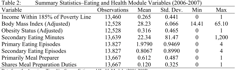
The U.S. Department of Agriculture in conjunction with the National Institutes of
Health-National Cancer Institute has delivered the Eating and Health Module (EH Module) of the ATUS
for the 2006 and 2007 cohorts. Because the ATUS only records primary activities, eating
concurrent with other activities–such as “snacking” while working or watching television–is
ignored. However, the EH Module addresses respondents’ secondary eating behaviors by
recording how many minutes respondents were eating during another primary activity. The EH
Module includes several additional items, including self-reported height and weight from which
body mass index (BMI) is calculated,7 respondents’ roles in household meal preparation, and
households’ relation to the poverty line.
The CPS provides numerous socioeconomic items. We include standard control
variables: age, gender, race and Hispanic status, education, marital status, number of children, an
indicator for the presence of a child 0-1 years, household income,8 disabled worker status, and
employment status. Employment status is disaggregated into broad occupation categories to
acknowledge physical exertion variation across occupations: “White collar” workers are those in
management, business, financial, and professional occupations; “Service” workers are those in
service, sales, or office administrative support occupations; and “Blue collar” workers are those
6 For further details, the reader is referred to Hamermesh et al. (2005), who write a descriptive overview of the
ATUS. One characteristic of the ATUS is low response rate (below 60%); there is no evidence that non-response is due to individuals being “too busy”, though nonresponse has been linked to weak community integration (Abraham et al. 2006). Additionally, ATUS respondents are found to have a greater propensity towards volunteering
(Abraham et al. 2009).
7 Body Mass Index is calculated as kg/m2. Individuals are defined as obese if their BMI is greater than or equal to
30. We correct self-reported height and weight with algorithms derived from regressing actual height and weight on reported height and weight from National Health and Nutritional Examination Survey data (for ages 21-65, only– other ages’ BMIs are recoded as missing).
8 Household income is reported by bracket set. We recoded income as the midpoint of the household’s income
from farming, fishing, forestry, construction, extraction, installation, maintenance or repair,
production, and transportation occupations. We additionally distinguish self-employed and
hourly workers who may have more and less flexible work schedules, respectively. We code an
indicator equal to one if the respondent is enrolled in school. We code an indicator variable
“smoker” equal to one if the respondent reported any time using tobacco (or marijuana) products,
which will proxy for some individual health preferences. We code a severe weather indicator
equal to one in instances in which rainfall equaled or exceeded 0.6” or snowfall equaled or
exceeded 0.1” inches on average over the respondent’s metropolitan area their diary day.9
I model time participation in four health-related activities: (1) aggregate exercise, which
is the summation of total time spent in thirty-five individual exercise and sport activities; (2)
total time spent preparing food; (3) the total time spent eating as a primary activity; and (4) total
time spent sleeping. We also model time socializing and watching television–which together
comprise two-thirds of Americans’ waking leisure time–as benchmark comparisons. We detail
all time variables’ construction in the appendix.
The analysis’s principal explanatory factor is time spent commuting. Modeling travel
behavior with the ATUS is difficult, as explained by Brown and Borisova (2007). The issue is
that the ATUS segments each travel episode by destination purpose. If a commuter brings a
child to school before traveling to work, the ATUS only categorizes the school-to-work portion
as work-related travel. The home-to-school portion is classified separately, even if it is a routine
occurrence that arguably should also be included as part of the “commute”. Ignoring such
segments means that the ATUS-tabulated “travel related to work” underestimates commutes for
individuals making stops between work and home–estimated at about one third of all commute
9 Weather data are from the National Climactic Data Center. “Average over the respondent’s metropolitan area”
trips (p. 10). To accommodate commuting trips with multiple purposes, We manually calculate
individual commute times from ATUS diary activity logs using Brown and Borisova’s definition
of a commute: all travel time for any purpose from the time the respondent leaves home until
arrival at work, and vice versa. A respondent’s total commuting time is the summation of all
qualifying travel time.10
Instrumental Variables
The survey’s cross-sectional design creates the primary impediment to causal inferences.
To mitigate selection bias, an ideal instrument set will explain the diary day’s commuting time
yet also be uncorrelated with health-related activity time. For most commuters, the degree of
traffic congestion is a primary determinant of the daily variation in time traveling between home
and work. The Department of Transportation reports the largest sources of congestion as
bottlenecks, traffic incidents, work zones, and poor weather. In terms of validity as instruments,
bottlenecks are non-random, weather conditions influence health-related time allocation, and to
our knowledge no nationally-representative dataset exists detailing construction zones by
location and day.
I focus on fatal traffic accidents to proxy highway congestion.11 Fatal accident
occurrences are exogenous to the individual and would create the magnitude of congestion that
would saliently impact traffic flow. We use fatal accident records from the Federal Highway
Administration’s Fatal Analysis Reporting System and aggregate hourly tallies by CBSA for
each diary day. We limit the recorded accidents to those occurring on National Highway System
roads during “rush hours”–between 6am-9am and between 4pm-8pm on non-holiday weekdays–
10 As Brown and Borisova (2007) acknowledge, this definition itself is problematic because the ATUS only records
one day and so the researcher cannot ascertain which stops are routine and which are not.
11 In addition to fatal accidents, we experimented with gasoline prices, hazardous material spills, annual
in order to more precisely match commuters and relevant incidents. We then match the daily
metropolitan accident counts to each individual’s geographical location (CBSA), diary date, and
the times of day in which the respondent was commuting.
I distinguish each accident by the time of accident occurred to construct two dichotomous
instruments: whether an accident occurred during the respondent’s journey from home to work
(the morning commute) in the respondent’s metropolitan area on their diary day, and whether an
accident occurred during the respondent’s journey from work to home (the evening commute).
This distinction is because accidents occurring during the morning hours may have a different
effect than evening hour accidents for two reasons: (1) the working population's shift towards the
urban core during work hours means that accidents occurring when the populace is more
centralized will affect more people in denser circumstances, and (2) the timing of the work day
may mean that one trip is more flexible than the other with regards to the journey’s timing,
allowing workers to adjust their departure times in case of (anticipated) congestion more for one
than the other, lessening any congestion impact.
Sample Construction and Summary Statistics
The full sample is constructed as follows: when ATUS samples from survey years 2003
through 2008 are aggregated, 85,645 observations comprise the full set. Given the focus on a
work-related activity–commuting–We limit the sample to working age (18-65) adults residing
within identifiable urban labor markets, specifically the respondent’s Core Based Statistical Area
(CBSA).12 These criteria result in the omission of 18,464 individuals from rural
(non-metropolitan) counties, and then 10,410 individuals outside of the age range. Next, individuals
12 A CBSA is a geographic entity defined by the U.S. Office of Management and Budget containing an urban core of
with incomplete records are dropped: 7,035 individuals with missing household income,13 an
additional 403 with missing weather data, and an additional 31 with missing occupational
categories are excluded.
Lastly, to construct a sample which permits meaningful comparisons and which will
produce inferences with reasonable generalizability, we limit the sample to individuals falling
under loosely-defined "traditional" commuting schedules. Essentially, night shift workers are
dropped. Commuters are eligible for inclusion if they arrived at work between 4:30am and 6pm,
and also arrived at home between 10am and 11:30pm. Moreover, any individual–working or not
working–identified as beginning or ending the day away from home is omitted. Together, these
criteria resulted in the loss of 2,810 further observations. The final dataset includes 46,496 full
observations.
The instrumental variables sample is further reduced. For this procedure, We omit the
32,005 non-commuters for two reasons: (1) traffic accidents are inapplicable to non-commuters,
and more importantly (2) selection into commuting arises from a decision to select into labor
force participation the specific diary day, an additional source of endeogeneity. Finding a factor
to explain the labor decision would likely encompass a catastrophic event such as severe weather
or illness which would also affect health-related activity time, invalidating the factor as an
instrument. Second, we omit the 741 commuters who did not use a car during any portion of
their commute, for whom traffic accidents are also irrelevant. Third, we omit 1,731 respondents
whose journey to work or returning home was less than ten minutes, as these individuals are least
likely to have used highway roads, where relevant traffic accidents took place.
13 In the sizeable number of observations with missing income data, 93.4% refused to provide the information, 6.4%
The remaining IV sample is reduced to 12,019, for which the instrument’s coverage is
limited–only approximately 1.33% of commuters qualified as having one or more fatal traffic
accidents occurring within their metropolitan area during rush hours on their ATUS diary day.
Moreover, although accidents occur everywhere, they are 1.26% more likely {p-value < 0.000}
in bigger cities (Atlanta, Boston, Chicago, Houston, Los Angeles, New York, Philadelphia, and
Phoenix), a particular segment of the sample distribution. Ultimately, however, results will be
conditional on CBSA, which captures location effects. However, because the impact of traffic
accidents may be more pronounced in larger often more congested cities, we employ a second IV
sample further restricted to residents of the fifteen most populous metropolitan regions.14 The
limited IV sample encompasses 4,282 observations.
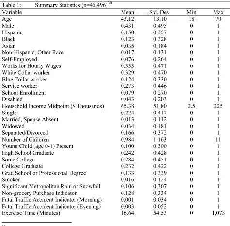
Full summary statistics are included in Tables 1 and 2. Table 1 presents summary
statistics for all ATUS variables and Table 2 lists summary statistics for variables taken from the
EH Module. Table 3 presents selected activity time-use averages for three particular types of
individuals within the ATUS sample: those with zero commutes, those ±10 minutes of the
50-minute daily commuting time median and those with total commuting times of 180 50-minutes or
greater, following the U.S. Census definition of an “extreme commuter”.15 We limit the “no
commute” group to those working (at home) at least four hours to provide a meaningful
comparison with commuters, who implicitly allocate time to labor. The fourth column reports
Analysis of Variance F-Statistics under the null hypothesis that activity means are equal across
commuting length groups.
14 The fifteen most populous regions, based on 2008 Census estimates, are New York, Los Angeles, Chicago,
Dallas, Philadelphia, Houston, Miami, Atlanta, Washington, Boston, Detroit, Phoenix, San Francisco, Riverside/Bernardino, and Seattle.
15 Approximately 2.23% of commuters in the ATUS sample spent 180 minutes or more of the diary day commuting,
Most activities decrease with commute time: extreme commuters sleep 44.7 minutes
(9.5%) less than non-commuters; they also spend 10.1% less time in primary eating, 38.3% less
time preparing food, and 63.3% less time exercising. Not all activities strictly decrease as
commutes lengthen–television watching rises then falls over commute length. Lastly, there is no
evidence of any significant difference in socializing time averages across groups. For all other
activities at least one group’s mean is significantly different.
Analytical Results
All regressions include labor market participation time, age, gender, race, ethnicity,
employment information, disability status, school enrollment, marital status and child
information, education, household income, smoking indicator, severe weather indicator, and
indicators for CBSA and ATUS diary date. There are time indicator variables coded for the day
of the week, the month, and the year of the ATUS diary day. There is also a holiday indicator
equal to one if the diary day coincided with New Year’s Day, Easter, Memorial Day, the Fourth
of July, Labor Day, Thanksgiving, or Christmas. We report standard errors clustered by
respondents’ CBSA in parentheses.16
OLS Results
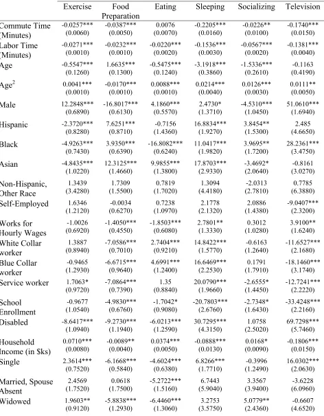
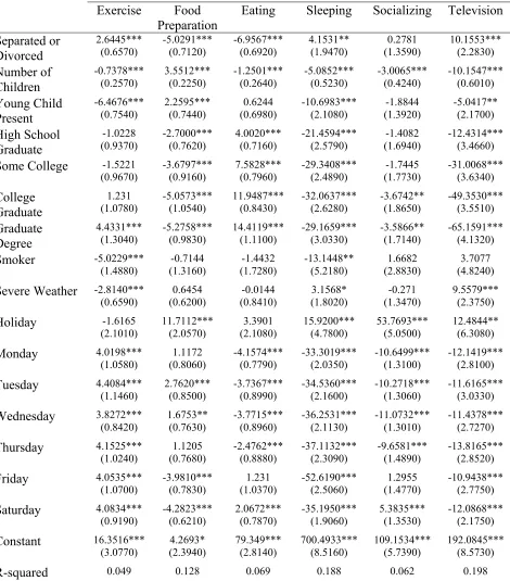
I report full ordinary least squares coefficients modeling activity time allocation in Table
4, where each column’s heading indicates the activity used as dependent variable. All time use
variables are in minutes, so coefficients on commute and labor time are interpretable as
per-minute trade-offs. There is evidence of strongly significant negative associations between
commute length and exercise, food preparation, sleeping, socializing, and television viewing
times. Each minute spent commuting is associated with a 0.0257 minute reduction in exercise
16 We also generate but do not report both unadjusted standard errors and Seemingly Unrelated Regression (SUR)
time, a 0.0387 minute reduction in food preparation time, a 0.2205, minute reduction in sleep
time, and comparatively a 0.0226 and 0.1740 minute reduction in times spent socializing and
viewing television, respectively. The largest estimated activity trade-off with commuting is with
sleep time; certainly, sleep-loss implications permeate many facets of life beyond nutritional
health outcomes.
Although highly significant, the coefficients are small in magnitude. The median 50
minute commuter loses only 1.29 minutes in exercise, 1.94 minutes of food preparation, and
11.03 minutes of sleep. However, these calculations are a single day’s trade-offs, only, and
effects may cumulate. The growth in obesity rates since the 1980s is equivalent to 100-150
additional calories per day–“three Oreo cookies or one can of Pepsi” (Cutler et al. 2003, p. 100)–
and so slight behavioral changes daily can produce dramatic results. Ignoring the extrapolation
and assuming moderate 280 calorie per hour exercise, an additional hour commute is associated
with a 1,414.6 lesser caloric expenditure due to lost exercise over a 235 working day year.17 If
short-run exercise differences are unsubstantial in the short-run, there are also additional
nutritional effects, evidenced by reduced food preparation time, which are unfortunately
impossible to precisely measure using ATUS data. Modest coefficients are also consistent with
the hypothesis that time constraints are a small but meaningful factor among an array of complex
causes determining health outcomes.
There is no significant evidence of a trade-off between commuting and primary eating
time. One interpretation for the absence of a significant association is that eating is a highly
valued activity and individuals resist allocating away eating time. Additionally, eating is
characterized by the ability to be performed concurrently with other activities and so eating time
is particularly prone to measurement error given that the standard ATUS only measures primary
activities. We analyze secondary eating time–and additional dietary behaviors–using the EH
Module in Section V below.
Comparatively, the labor time coefficient is consistently significantly negative across
activities, suggesting that there is also a negative trade-off between labor time and health-related
activities. In particular, these findings support Ruhm’s (2005) explanation of improved health
outcomes in economic downturns due to recovered leisure time resulting from unemployment.
In comparison to the commuting time coefficient, the labor time coefficient is statistically
indistinguishable for exercise {p-value = 0.8071}, but the commuting coefficient is statistically
greater in magnitude than the labor time coefficient with respect to food preparation {p-value =
0.0053}, sleep {p-value = 0.0001} and television times {p-value = 0.0247}. On a per-minute
basis, commuting is associated with a greater amount of time traded-off with these activities than
labor time is. The exception is time spent socializing, where the trade-off with labor time
exceeds that with commuting time {p-value = 0.0001}.18
Lastly, the comparative coefficient magnitudes across activities suggest the limited health
impact policies solely seeking to reduce commute (and labor) time might have–a one-minute
reduction in commute time increases television watching over six times more than it increases
exercise. The inefficiency of such a policy is measureable by the degree to which time savings
are diverted into activities unproductive to health. An effective policy should also channel
reclaimed leisure time specifically into health production.
18 One of Putnam's (2000) principal inferences is that solitary commuting results in fewer social interactions and
Active and Sedentary Commuting Mode Comparisons
A valid critique of the commute measure is that respondents engaged in utilitarian
exercise–walking or cycling as a transit mode19–bias coefficients. Individuals with longer
active-mode commutes will need less non-travel exercise, but it would be incorrect to
characterize their exercise trade-off with commuting as unhealthy since some exercise is
achieved via transit. There is legitimate potential for bias: 10.9% of ATUS commuters reported
some active commuting portion, and 3.8% reported active commuting portions of thirty minutes
or greater. Because the ATUS identifies mode of transportation, we disaggregate total commute
time into an active portion and two sedentary portions–“engaged” and “passive”–to separate this
confounding factor. The active mode portion is total minutes of the commute spent walking or
cycling, the “engaged” sedentary mode portion is total minutes spent operating a vehicular mode
(such as driving a car), and the “passive” sedentary mode portion is total minutes spent as a
non-operating passenger of a vehicular mode. The motivation for separating engaged and passive
sedentary modes is that for some public transit users, commuting time is highly productive (with
regards to work or certain leisure activities), which may free up time for health-related activities
more than those employing engaged sedentary modes. We present commute time coefficients
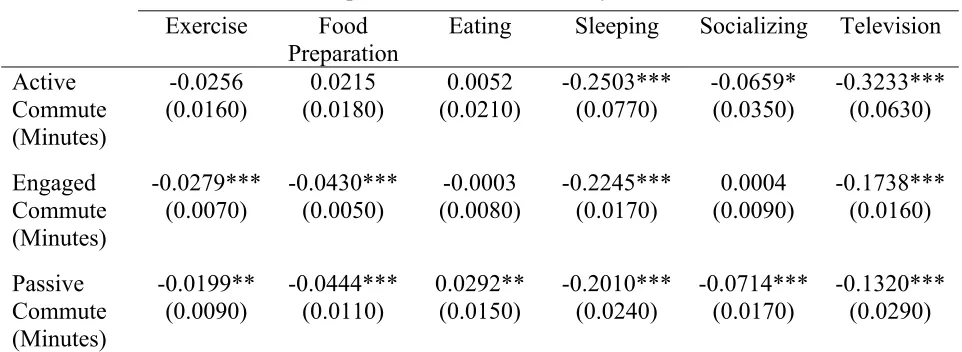
disaggregated by both active and sedentary mode usage times in Table 5.
With respect to exercise, the time trade-off appears to come entirely from sedentary
commuting. Both of the sedentary commuting coefficients are significant, though statistically
indistinguishable {p-value = 0.3797}. Despite the expected bias from utilitarian transit, there is
no evidence of a significant trade-off between exercise and active commuting. Individuals do
not consider active commuting a form of utilitarian exercise to the extent that it crowds-out
non-
19 Using active modes of travel is a commonly-prescribed solution in the popular media for individuals who feel
travel exercise behaviors. Similar to exercise, only sedentary commuting time coefficients are
significant with respect to food preparation.
Disaggregation reveals significant associations between commuting and eating time,
whereas the aggregated commuting time coefficient is insignificant. Specifically, the passive
commuting time coefficient is significantly positive–perhaps passive commuters apply time
saved by in-transit productivity towards traditional sit-down meals. It is less clear why only
passive commuting–and to a weaker extent active commuting–affects socializing time. One
possibility is that passive commutes allow unrecorded secondary socializing opportunities which
are not characteristic of engaged commuting.
For sleeping and television times, the coefficients on active and both sedentary commute
times are significant. Moreover, for television the active commuting coefficient exceeds the
sedentary commute modes’ coefficients in magnitude {p-value = 0.0402}. One explanation is
that active commuters have less affinity for and are more willing to trade off sedentary activities
such as watching television, which illustrates the potential endogeneity inherent in modal choice.
The commute mode coefficients are statistically indistinguishable for sleeping {p-value =
0.6366}.
Censored Regression Results
All time participation dependent variables are constrained to the twenty-four hours
observed in the diary day. Previous time-use analyses often employ Tobit models to
accommodate censoring of activity times, while other researchers propose that OLS is adequate
from observational windows which are too brief or whether they represent true
nonparticipation.20
For comparison, we calculate censored-regression coefficients for exercise, food
preparation, eating, and sleeping activities. All regressions are left-censored at 0; there are no
activity participation observations at the upper bound of 1440 (total minutes in a day) and so
right-censoring is unnecessary. Table 6 displays marginal effects, calculated as the change in
activity time conditional on being uncensored, for commute time–both aggregated and
disaggregated into active and sedentary portions–and labor time.
After accounting for censoring, most of the relationships from OLS results remain with
slight changes in magnitude: each minute spent commuting is associated with a 0.0294 minute
reduction in exercise time, a 0.0295 minute reduction in food preparation time, and a 0.2203
minute reduction in sleep time. Commuting time is again insignificant with respect to eating
time. When commute time is disaggregated, again only sedentary commuting modes are
significant with respect to exercise time, only passive commuting is associated with eating time,
and both active and sedentary commuting time are significantly related to sleep time. The
primary difference from OLS results is that the censored-regression active commuting
coefficient is now weakly positively significant for food preparation. One explanation for this
also involves transit mode self-selection: individuals who actively commute are more
health-conscious and invest greater amounts of time in (healthy) meal preparation.
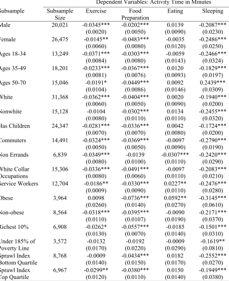
Commute Time Coefficients by Sample Stratifications
Table 7 presents OLS coefficients for commute time with respect to exercise, food
preparation, eating, and sleeping time stratified by different subsamples to identify differences in
20 Foster and Kalenkoski (2008) provide a succinct overview of the OLS-vs-Tobit debate and empirically illustrate
commuting time response among different populations. The subsamples we analyze are: males,
females, three age groups (respondents aged 18-34, 35-49, and 50-70), white, nonwhite,
households with children, commuters only, “non-errand” commuters (commuters making no
stops between home and work), white collar employees, service occupation workers, the obese,
the non-obese, households above 90th percentile income, and under 185% of the poverty line.
We also utilize the Smart Growth America metropolitan sprawl index–first used by Ewing et al.
(2003) to link obesity and urban sprawl–to investigate whether the commuting time-use
trade-offs vary over urban form.21 We group the bottom quartile of the sample with respect to the
sprawl index, which by the index’s design are residents of the most sprawled metropolitan areas,
and the top quartile of the distribution (the residents of the least sprawled areas).
Subsample results suggest that males trade off exercise with commuting more than
females (coefficients are -0.0345 and -0.0145), but females trade off food preparation more than
males (coefficients are -0.0202 and -0.0483). The exercise trade-off with commuting decreases
with age, the food preparation trade-off increases with age, and sleep trade-off dips in middle age
and then rises. White respondents trade off exercise while there is no evidence that nonwhites
do, and non-obese individuals trade off exercise while there is no evidence that obese individuals
do. The commuting coefficient is significant the greatest number of occurrences within the
sleeping time category–in all fifteen subsamples–and is significant for the least number of
coefficients (three of the possible fifteen) within the eating time category.
21 See www.smartgrowthamerica.org. The index is constructed so that lower values indicate areas of greater urban
When commuting is significant within the eating category, it is positive for service
workers and the obese. Given the relationship between caloric intake and obesity, there may be
certain individuals who react to longer commutes by spending more time eating–perhaps in
response to commuting stress–which leads to weight gain. In contrast, the commuting
coefficient is significantly negative for the subsample of those commuting directly between
home and work. Perhaps the decision to run errands as part of a commute is also influenced by
unobservable individual characteristics.
One noticeable result is the magnitude of the coefficient within the food preparation
category for the obese subsample, which at -0.736 exceeds every other subsample’s coefficient.
Perhaps obese individuals are most willing to trade off food preparation time for commute time,
due to some inherent trait. If foods requiring less preparation time also promote obesity, this
effect will self-reinforce. Additionally, those in the bottom quartile of the Smart Growth sprawl
index–residing in the most sprawled areas–trade off food preparation for commuting more than
individuals residing in the least sprawled metro areas. This finding is consistent with a
hypothesis that obesity is higher in areas of greater sprawl because individuals preferring low
time cost, less nutritious meals self-select into these areas.
Instrumental Variables Results
To circumvent self-selection bias, we incorporate fatal traffic accidents as exogenous
factors increasing commute time into the analysis. We display first stage results in Table 8
detailing metro-area fatal traffic accidents’ effect on commuting time. Both accident indicator
coefficients are significantly positive, as expected–traffic accidents proxy congestion which
lengthens travel time. A morning incidence of a metropolitan-area fatal traffic accident is
a 14.9 minute longer commute. The F-statistic testing the instruments’ joint contribution to the
model is 10.96 {p-value < 0.0000}, satisfying the greater-than-10-F-statistic rule-of-thumb for
sufficiency (Staiger and Stock 1997).22
Table 8 also presents commuting time OLS coefficients using the reduced sample,
commuting time IV coefficients, and both the χ2 and F-statistics from and J-Hansen and
Durbin-Wu-Hausman tests (with p-values in braces), respectively. The J-Hansen over-identifying
restriction tests demonstrate that fatal traffic accidents are inappropriate for use as instruments
when modeling eating time. In turns out that incidence of an evening accident is associated with
6.79 additional minutes of eating per day {p-value = 0.0233}.23
If using accidents as instruments yields consistent estimators, then the
Durbin-Wu-Hausman tests indicate that endogeneity bias does not statistically influence OLS commuting
coefficients’ estimates in the full IV sample, and so using OLS results is appropriate. It may be
that combinations of control variables, including the smoking and disability indicators, proxy for
unobservable health preferences, the theoretically confounding factor. Future work should
particularly seek to identify additional instruments or alternative identification strategies to
compare results.
For sleep time, the Hausman test almost passes weak evidence of endogeneity and
moreover among the four outcomes sleep time is the only activity for which the commuting IV
coefficient is significant {p-value = 0.1294}. Interestingly, the IV coefficient point estimate is
more than double in magnitude that of the OLS estimate, suggesting that a one-minute increase
22 The severe weather indicator, although not a valid instrument, is also a random external factor potentially
influencing traffic. Unreported results indicate the coefficient if positive as expected–a value of 0.3350–but insignificant {p-value = 0.784}. It may be that the thresholds used to code the variable are insufficient to affect travel speed. The weather variable is also more weakly matched to individuals, since unlike traffic accidents it is not possible to tie weather conditions to specific times of the day.
23 When incidence of a morning accident is alone used as a single instrument, the Hausman test fails to demonstrate
in commuting time decreases sleep time by 0.7499, and the commuting IV coefficients for
exercise and food preparation times similarly increase in magnitude, although insignificant. This
is unexpected because the theoretical bias–location self-selection by health preferences–increases
coefficient magnitudes. IV coefficients should then be of lower magnitude, not greater.
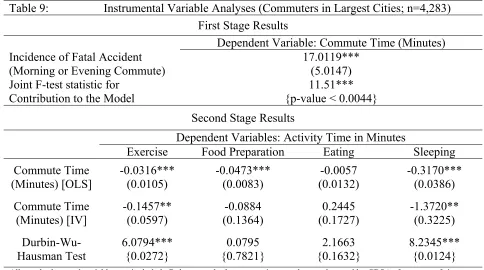
Table 9 displays estimates using the sample of commuters in the fifteen most populous
metropolitan areas. Morning and evening accidents are now combined into a single diary day
accident indicator to accommodate the smaller sample size and still produce a joint F-statistic
greater than ten. In first stage results, a fatal traffic accident occurrence is associated with an
additional 17.01 minute daily commute. In second stage results, there is now Hausman test
evidence that endogeneity bias affects the commuting time coefficients for exercise and sleep
time. As in the full IV sample, reduced sample IV coefficient magnitudes increase: an additional
minute of commuting is associated with 0.1457 fewer minutes exercise and 1.3720 few minutes
sleep time. The IV coefficient’s point estimate under sleep is less than “-1”–implying that
indirect effects are present since the associated sleep loss exceeds the one-minute attributable to
commuting time –although the estimate is not statistically different from negative one {p-value =
0.5319}.
The populous metropolitan area sample reinforces the evidence of increased trade-offs
between commuting and both exercise and sleep time. Consistent with predictions of Becker’s
(1965) composite good theory, these time-intensive activities might be particularly prone to
increased time constraints relative to food preparation and eating, which involve relatively more
monetary good inputs. Given the theoretical direction of the endogeneity bias due to
unobservable preferences, future research should seek to replicate these findings, to ensure their
One alternative possibility is that individuals respond to lengthened commutes due to
congestion differently than they respond to more typical commuting portions. Time spent stalled
in traffic might increase stress disproportionately to typical commuting time, debilitating
commuters’ willingness to engage in health-related activities and consistent with the increased
IV commuting coefficient magnitudes. It is not possible to directly measure stress in the ATUS;
however, the survey does capture time spent in sleeplessness, which may proxy for stress levels.
Neither morning {p-value = 0.9364} nor evening {p-value = 0.4756} traffic incidences are
significantly associated with increased sleeplessness, so there is no empirical evidence of bias,
though future research must consider of instrumental variables’ potential indirect effects.
Measuring commuting time’s indirect effects will enable a more definitive understanding of the
mechanisms influencing health-related activity time reductions.
Tests and Extensions
MET Analysis: An Examination of Physical Activity Intensity
Caloric expenditures vary by activity. If longer commutes are physically draining, one
potential byproduct from traveling is that individuals substitute into less intensive activities
resulting in reduced energy expenditure for a given quantity of exercise time. To test this
possibility, we match activity times to MET intensity values Tudor-Locke et al. (2009) construct
for ATUS activity categories to calculate MET minutes. A “MET” (or “metabolic equivalent”)
is a unit commonly used to gauge the intensity of a physical activity and “MET minutes” are the
minutes spent in an activity multiplied by that activity’s MET value. A MET is defined as the
ratio of energy expenditure in an activity to expenditure at rest.24 For example, a MET value of
2.0 indicates that the activity requires twice as much energy than if the person were resting. The
24 A MET value of 1.0 is equivalent to a metabolic rate consuming 3.5 milliliters of O
ATUS MET values range from the low of 0.92 (sleeping) to 10.0 (doing martial arts or playing
rugby).
Using these intensity values, we calculate “MET minutes”, defined as individual i’s
participation in activity k weighted by k’s MET intensity, summed over a set of activities:
s time in activity MET intensity for activity
We construct two MET minute indexes: the first where K is limited to ATUS exercise
activities only and a second where K is limited to all other non-exercise leisure activities day.
We use exercise MET minutes as an outcome variable regressed on commuting time (and all
other factors). MET minutes combines time in activities with the activities’ degree of
strenuousness and thus roughly proxies caloric expenditures. We then include aggregate time
spent exercising as an additional control and regress again. MET minutes are the aggregated
product of activity time and strenuousness, or alternatively, MET minutes are average MET
values weighted by activity time participation. Therefore, holding time constant investigates
regressor associations with average strenuousness of the set K. While Table 4 regressions
analyze quantity of exercise, regressing exercise time augmented with MET intensity analyzes
quality of exercise. We then repeat the substitution test using the set of non-exercise leisure
activities to test for associations between lengthier commuting times and substitution into less
strenuousness non-exercise time uses. We display coefficients for pooled and disaggregated
commute times, labor time, and exercise/leisure time controls in Table 10.
The first three columns of Table 10 use exercise MET minutes as an outcome variable.
The first column’s significantly negative commute time coefficient shows that lengthier
commutes are associated with lower MET minutes. In the second column we control for
time. In this instance, commute time maintains negative significance, and so there is significant
evidence that commuting induces substitutions into lower exercise intensities, because longer
commutes are associated with lower average MET values, holding exercise time constant. This
result is consistent with the hypothesis that longer commutes produce a lethargic side effect. An
additional 41.7 minutes of commuting is associated with exercising on average intensity one
MET lower. There is no evidence of an analogous substitution due to labor time. The third
column repeats the second column’s model with commuting time now disaggregated by active,
engaged, and passive transit modes. There is no evidence that walking or cycling is associated
with substitution into lower intensity exercises, but there is weak evidence that engaged mode
and strong evidence that passive mode commuting times are associated with lower-intensity
exercises. An additional 16.47 minutes only of passive commuting is associated with exercising
at an intensity level an average of one MET lower.
In the fourth column, the set of k is all non-exercise activities; commute time is
disaggregated by mode and non-exercise leisure time is held constant. All commute and labor
time coefficients are significantly positive. This suggests that the average strenuousness level of
non-exercise activities increases with both commuting and labor time. The active commuting
time coefficient point estimate is the largest, although all commuting mode coefficients are
statistically indistinguishable {p-value = 0.4695}. The labor time coefficient, however, is
statistically distinct from the commuting coefficients {p-value < 0.0000}.
Is it possible that commuting and labor produce an invigorating effect which increases
non-exercise activity intensity? Two alternative possibilities are (1) that individuals manage
their schedule so that work day leisure activities are busier and more strenuous, days off from
activity arrangement. Additionally, (2) because sleeping and television–inherently sedentary
time uses–are the activities most traded off with commuting and labor time, their trade-off raises
the non-exercise leisure time average MET intensity score. An interesting extension would
transpose MET minutes to caloric expenditures and calculate net caloric expenditures associated
with commuting time.
An Extension to Analyses of Eating and Food Preparation Behaviors
Commuting is consistently insignificant with respect to eating behavior in pooled
samples. However, primary eating time is particularly prone to measurement error due to
omitted secondary eating–time spent eating while engaged in another primary activity. The EH
Module indicates a non-trivial amount of secondary eating–respondents’ average time spent
eating secondary to another activity was 22.34 minutes, or 18.7% of the total minutes they ate.
Although the data do not show an association between commuting and primary eating, it is
possible that commuting affects secondary eating time, for instance by providing an
environment–such as a car–in which to snack. To test this hypothesis, we utilize the EH
Module’s secondary eating information. We regress secondary eating time in minutes on
commuting time and labor time (here both scaled to hours). OLS results are in the first column
of Table 11.
EH Module data do not demonstrate any evidence of an association between total
secondary eating and either commuting or labor time. It appears that neither commuting nor
work time are associated with differences in eating time in either traditional meal settings or
while concurrent to other activities. These results may be moot, however, given evidence that
the frequency of eating episodes–not the minutes spent eating–explains ATUS respondents’ BMI
Certainly, time constraints imposed by longer commutes might force individuals to eat fewer
meals throughout the day.
To test this possibility, we examine whether commuting time is associated with the
number of diary day primary and secondary eating episodes.25 Negative binomial regression
coefficients are presented in the second and third columns in the top half of Table 11. The
coefficients on commute time are insignificant for both primary and secondary eating episodes–
there is no evidence of an association between time spent commuting and the number of meals
throughout a day. The coefficient for labor time, however, is positively (weakly) significant with
respect to primary eating episodes. Recalling that in Table 4 there is a negative relationship
between labor and primary eating times, the overall evidence suggests greater labor time is
associated with less primary eating time overall, but with more meals throughout the day, and
does not influence secondary eating behaviors.
Although eating time is not associated with commuting time, increased time constraints
due to commuting might influence the type and health quality of meals prepared and consumed,
especially given that the ATUS demonstrates a trade-off between commuting and food
preparation times. Reduced food preparation time resulting from lengthier commutes may
increase the consumption of pre-prepared, often less-healthy meals obtained from either full- or
limited-service food establishments. To further investigate this, we code an indicator variable
equal to one if the respondent reported any time spent purchasing non-grocery food items.26
Probit regression marginal effects using this indicator as the dependent variable are presented in
the bottom half of Table 11. Each probit regression’s sample is differentiated by self-reported
25 Primary and secondary eating episodes are coded as having four if the number reported was four or greater; this is
approximately the top 1% of each distribution.
26 The indicator is constructed as equal to one if ATUS variable t070103, indicating minutes spent “purchasing food