Wavelet estimation of copula function based on cencored data

R E S E A R C H

Open Access

Wavelet estimation of copula function based

on censored data

Bahareh Ghanbari

_{, Masoud Yarmohammadi}

_{, Narges Hosseinioun}

_{and Esmaeil Shirazi}

*_{Correspondence:}

[email protected] 1_{Department of Statistics, Payame}

Noor University, Tehran, Iran Full list of author information is available at the end of the article

Abstract

In this paper, we consider wavelet analysis to obtain an estimator of a copula function based on censored data. We show that optimal convergence rates for the mean integrated squared error (MISE) of linear wavelet-based function estimators are exact under right censoring model. Moreover, we derive asymptotic formulae for MISE. Finally, the simulation results and the analysis of real data validate the proposed procedure.

Keywords: Censoring; Copula function; Kaplan–Meier estimator; Nonparametric estimation; Ranks; Wavelet estimators

1 Introduction

Recently, copulas and their applications in statistics have become a rather popular phe-nomenon. For a long time, statisticians have been interested in the relationship between a multivariate distribution function and its lower-dimensional margins. When it comes to analyzing the dependence between random variables, the copula function becomes a very useful tool. According to Sklar’s theorem [22], ifHis a bivariate distribution function with marginsF(x) andG(y), then there exists a copulaCsuch thatH(x,y) =C(F(x),G(y)). Statisticians are interested in copulas for two reasons: (1) Inspecting how the measures of dependence are scale-free and (2) constructing families of bivariate distributions. For more information about this flexible tool and dependence modeling, we refer to [16] and [20]. A detailed survey on copula models can be found in [24]. Copula models have many applications in finance and insurance, some of which are considered in [2,7,10,11,13]. For more studies on copulas in econometrics, we refer to [3] and [21].

In recent years, the analysis of censored data has become very popular. In many sci-ences such as statistics, engineering, finances, and other areas, censoring is a condition in which observation is partially known, that is, censoring occurs when a value is outside the range of a measuring instrument, particularly in life-testing data in medicine, where observations often survive or fail at the end of the test (see, e.g., [12] for good examples of the censoring method). LetT1,T2, . . . ,Tnbe i.i.d. survival times with probability den-sity functionf and common distribution functionF. Typically, instead of observing the variables of interest, we are able to observe the i.i.d. censoring timesC1,C2, . . . ,Cn. LetG be the common distribution function of the latter. Also, it is assumed thatTiandCiare

independent. LetYi=min(Ti,Ci) fori= 1, . . . ,n, and define the indicator function

δi=

⎧ ⎨ ⎩

1 ifTi≤Ci,

0 ifTi>Ci.

This definition denotes the right-censoring. Several approaches have been proposed to deal with the estimation of copulas under uncensored or censored data. See [9] for non-parametric estimation and also [23]. In [24] consistent estimators are considered under some restrictions on the dependence structure of the censored data. For right-censored data, less work has been done on nonparametric copula estimators. Recently, in [15] a new class of nonparametric estimators of copula function for bivariate censoring is described. The aim of this paper is to estimate the copula function via wavelets based on censoring. The theory of wavelets and their applications in statistics and other sciences have be-come an important technique. We can find several applications of wavelet estimators for copula functions in different contexts. In [14] smoothed empirical copula estimators con-sidered using ranks and wavelets. See [1] for more information about the procedure to estimate copula functions using wavelets, where the problem of multivariate copula den-sity estimation by wavelet methods has been described. In [19] the wavelet approaches were used, basically following the same route as in [14]. In [5] multiwavelets for estimat-ing copula density were used, and in [6] the same work was prepared based on a Legendre multiwavelets. There are many different papers that considered wavelets, and we proposed some of the most important.

Currently, an extension of wavelets and copulas is increasingly popular as an alterna-tive to many methods such as those briefly discussed. In this paper, we propose a lin-ear wavelet-based estimation for copulas with right censored data in the observationT1 orT2. Let (T11,T21), . . . , (T1n,T2n) be independent and have a joint distribution function (d.f.)F(t1,t2). As usual, assume thatT1andC1are independent, whereC1is the censoring variable associated with the variableT1. Rather than observing the variables of interest (T11,T21), . . . , (T1n,T2n), in the randomly right censor model, (Yi,δi,T2i) is observed. We apply the method of [17], which provides a MISE expansion similar to a density function over (–∞,T] for any fixedT <τH(·,t), whereτH(·,t)=inf{u:H(u,t) = 1} ≤ ∞is the least upper bound for the support ofH(·,t), the distribution function of (Z1,t).

The rest of the paper is as follows. In Sect.2, we define the elements of copula density and wavelet transform and provide the wavelet estimators for the copula based on the censored data. The main results are described in Sect.3, and the simulation study for the proposed estimator is provided in Sect.4. The proofs are presented in theAppendix.

2 Preliminary notations

In this section, we provide some necessary concepts about the general framework of this paper. Section 2.1presents preliminary assumptions and some notations about copula functions. All the major definitions and facts about the wavelets used in the paper are presented in Sect.2.2. At the end of the section we introduce the estimators for the main result.

2.1 Copula function

of the results to higher dimensions is straightforward. Consider a random vector (T1,T2) with cumulative distribution functionF(t1,t2) =P(T1≤t1,T2≤t2) and margin distribu-tion funcdistribu-tionsF1andF2. The relation between these variables is of interest, so the copula functionCcan be formed as follows:

F(t1,t2) =C

F1(t1),F2(t2)

.

The marginals F1 and F2 have uniform distribution on (0,1), and if they are continu-ous, then Cis unique and coincides with the distribution function of the pair (U,V) = (F1(T1),F2(T2)). In practice,Fis unknown. The advantage of using copula is that the joint distribution function (F(t1,t2)) can be constructed by using marginals (F1andF2) when they are from different classes of distributions. Let (T11,T21), . . . , (T1n,T2n) be a random sample from the unknown distributionF. Denote byF1nandF2nthe empirical distribu-tions associated withF1 andF2. A first step in selecting an appropriate class of copulas consists of plotting the pairs (Ri

n, Si

n) = (F1n(T1i),F2n(T2i)),i={1, . . . ,n}.

HereRiis the rank ofT1iamongT11, . . . ,T1n, andSiis the rank ofT2iamongT21, . . . ,T2n. The motivation behind this approach is that the pseudo-observations (Ri/n,Si/n) are close substitutes to the unobservable pairs (Ui,Vi) = (F1(T1i),F2(T2i)) forming a random sample fromC. We denote byc(u,v) the density ofC(u,v),

c(u,v) =∂ 2_C(u,v)

∂u∂v , u,v∈(0, 1).

It is obvious that in real analysis one of our variables (or even both of them) may be subject to be censored, and one observes a minimum between it and another (censoring) random variable, denoted byCj, soYj=min(Tj,Cj) andδj=ITj≤Cj forj= 1, 2. The i.i.d. replication

vector (Y1i,Y2i,δ1i,δ2i)1≤i≤ndenotes the random sample of (Y1,Y2,δ1,δ2). Clearly, many dif-ferent estimators can be considered for a distribution function based on censoring. The one used in this paper has the form

ˆ

Fn(t1,t2) = 1

n

n

i=1

W_in(·)I(Y1i≤t1,T2i≤t2),

whereWinare random weights designed to compensate asymptotically the bias caused by censoring and can be assumed in three different forms; see [15]. The weight considered in the present paper is

Win=

δ1i

1 –Gˆ(Y– 1i)

.

In this form onlyT1is assumed to be censored, and thenY2=T2,δ2= 1 a.s., andC1is in-dependent fromT1. AlsoGˆ, the Kaplan–Meier estimator of the censoring variable, is de-fined asGˆ(t) = 1 –_i:Y1i≤t(1 – n 1

j=1I(Y1j≥Y1i))

1–δ1i_{. IntroducingG(t) =P(C}

1≤t), the weight

Wincan be seen as an approximation ofWi=_1–Gδ1_(Yi–

1i). The other weights are discussed in

2.2 Wavelets

Wavelets and their applications are still an important subject in statistics. The term wavelet is used to refer to a set of orthonormal basis functions generated by dilation and translation of a compactly supported scaling function (father wavelet)φ and a mother waveletψassociated with anr-regular (r> 0) multiresolution analysis ofL2(R), the space of square-integrable functions on the line. Define φj,k(x) = 2j/2φ(2jx–k) and ψj,k(x) = 2j/2_ψ(2j_{x–k) forj∈Nandk= (k1,k2)∈Z}2_{. It is assumed thatj≥j}

o for some coarse scalejo∈N, which we take asl. We suppose thatφ andψ are bounded and compactly supported. For more on wavelets, see [8] and [18]. The wavelet expansion forf(x,y) can be written as

f(x,y) =fj0(x,y) +Dj0f(x,y), x,y∈R, (1)

wherefj0(x,y) = k∈Z2αj0kφj0k(x,y) is a trend of an approximation, and

Dj0f(x,y) =

∞

j=j0

k∈Z2

β_j(1)

0kψ (1) j0k(x,y) +

k∈Z2

β_j(2)

0kψ (2) j0k(x,y) +

k∈Z2

β_j(3)

0kψ (3) j0k(x,y)

.

For more details aboutDj0f(x,y) and the functionsψj0k, see [14]. The coefficientsαj0kand

β_j(1)

0k,β (2) j0k,β

(3)

j0k are unique for everyj0∈N. The functionφj0k is defined as φj0k1k2(x,y) =

φj0k1(x)φj0k2(y).

Some important cases of wavelets are the Haar, Daubechies, Shannon, Meyer, and Mor-let waveMor-lets (see [8]). We used the Haar and Daubechies wavelets in our simulation studies. Accordingly, by equation (1) the copula densityccan be expanded with

αj0k=

(0,1)2

c(u,v)φj0k(u,v)du dv, k∈Z2.

By the change of variablesu=F1(t1) andv=F2(t2) we get

αj0k=

φj0k

F1(t1),F2(t2)f(t1,t2)dt1dt2=Ef

φj0k

F1(T1),F2(T2). (2)

Assuming that I=I(Y1i≤T,T2i≤T), whenF1 andF2(the marginal distributions) are known, a moment-based estimator ofαj0kbased on censored data is then given by

ˆ

αj0k=

Iφj0k

F1(y1),F2(t2)

_ˆ

F(dy1,dt2)

=1

n

n

i=1

W_in(·)I(Y1i≤t1,T2i≤t2)φj0k

F1(Y1i),F2(T2i)

. (3)

Then the wavelet-based estimator ofcis given by

ˆ

cj0(u,v) =

k∈Z2 ˆ

WhenF1andF2are unknown, their empirical distribution functionsF1nandF2nare used. So the rank-based estimator is as follows:

˜

αj0k=

Iφj0k

F1n(y1),F2n(t2)

_ˆ

F(dy1,dt2)

=1

n

n

i=1

W_in(·)I(Y1i≤t1,T2i≤t2)φj0k

F1n(Y1i),F2n(T2i)

. (4)

Now we can introduce the linear wavelet-based estimator ofcbased on the ranks as

˜

cj0(u,v) =

k∈Z2 ˜

αj0kφj0k(u,v), u,v∈(0, 1). (5)

When we have no censoring, the definition reduces to that of the copula estimator in-troduced in [9]. We further denote by K any constant that may change from one line to another, does not depend onj,k,n, but depends on the wavelet basis and onc∞=

sup_{(u,v)∈(0,1)}|c(u,v)|andc2=c(u,v)2_{du dv.}

Since we deal with the wavelet method, it is very common to consider Besov spaces as functional spaces because they are characterized in terms of wavelet coefficients as follows. Besov spaces depend on three parameterss> 0, 1 <p<∞, and 1 <q<∞and are denoted byBs

pq. Letf ∈L2(Rd) (that is,L2(R2) in our paper), and lets<r(wavelet regularity). Define the sequence norm of the wavelet coefficients of a functionf∈Bs

pqby

|fBspq|=

k∈Z2 |αj0k|

p

1/p

+

j≥j0

2j0(s+d(1/2–1/p)) k∈Z2

|βj,k|p

1/pq1/q ,

where (|βj,k|p)1/p= ( k∈Z2 _∈S 2|βj,k|

p₎1/p_{. We assume that the copula functioncbelongs}

to a Besov space.

3 Main results

In this section, we present the main results. The following theorems show that the wavelet-based estimators wavelet-based on censoring attain nearly optimal convergence rates over a large range of Besov function classes. We also show that our estimator obtains the optimal vergence rates under mean integrated squared error (MISE) by accepting some mild con-ditions. The mean integrated squared error (MISE) is defined by

MISE(c˜j0,c) =Ef

1 0 1 0 ˜

cj0(u,v) –c(u,v)

2

dv du

.

In view of decomposition (1) forc, it is obvious that

MISE(˜cj0,c) =MISE(˜cj0,cj0) +

1

0

1

0

Dj0c(u,v)

2

dv du.

The bias term in the equation can be bounded as in the proof of Lemma 1 in [4],

1

0

1

0

Dj0c(u,v)

2

Precisely, suppose thatcbelongs to the ball of radiusM> 0 in the Besov spaceBs p,q(M), where the parameterss> 0 andp≥2, 1≤q≤ ∞ors> 2/p– 1 andp∈[1, 2], 1≤q≤ ∞; also,s∗can be defined ass∗=s+ 1 – 2/pifp∈[1, 2] ands∗=sotherwise. Also, by defining ˆ

cj0 based on Eq. (3), we can easily show that

MISE(c˜j0,cj0)≤2MISE(˜cj0,cˆj0) + 2MISE(cˆj0,cj0).

We now look for an optimal upper bound for each of the above sequences.

Lemma 1 Letαˆbe as in(3),and let j0be an arbitrary integer inN.Then

S1≡E

k∈z2

(αˆj0k–αj0k) 2_≤K

1 22j0

n

for some constant K1> 0depending only onφand either

c2=

c(u,v)2du dv or c∞= sup

u,v∈(0,1)

c(u,v).

Also note that the proposed linear wavelet estimator of cj0 isˆcj0(x,y) = k∈Z2αˆj0k×

φj0k(x,y). Then

MISE(cˆj0,cj0) =O

22j0

n

.

Note thatj0must be chosen so that 2j0 √

n.

Proof of Lemma1 The proof is similar to optimality results in Sect. 5 of [14].

Theorem 1 Assume that the functionφis m-differentiable,and letc˜j0be the copula density

estimator of c defined in(5). Then there exists a constant K1> 0such that, for a given (u,v)∈(0, 1)2and any level j0satisfying2j0(n/logn)1/2–1/2m,

MISE(c˜j0,cˆj0)≤K1 22j0

n

22j0logn

n + 2

–j0_logn

.

The error term associated with the use of ranks is negligible with respect to the usual error term as soon as 2j0_{log(n). For the proof, see theAppendix.}

Now, combining the results of Lemma1and Theorem1, we are in a position to express the main theorem of this section.

Theorem 2 Letφbe a scaling function mentioned in Sect.2.2having m derivatives with m> 1 + 1/s∗,and for arbitrary j0∈N,letc˜j0 be the estimator in(5).Then there exists a

constant K2> 0such that,for all M∈(0,∞),s> 2/p– 1,and p,q∈[1,∞),if j0 satisfies 2j0_n1/2+2s∗_,then

sup

c∈Bsp,q(M)

Note that the procedure of estimation described is optimal on the Besov space. The simulation studies are applied in the next section. For the proof, see theAppendix.

Remark1 This study can be regarded as an extension from complete data to randomly

right censored data. If we assume that there is no censoring, that is,G≡0 on (–∞, +∞), thenδ1i= 1 for alli= 1, 2, . . . ,n, and the estimators defined by (4) and (3) are the same as those of [14] for the complete data case. Therefore our estimators can be regarded as an extension of those of [14] from complete data to randomly right censored data.

4 Simulation studies and analysis for real data

In this section, we conduct simulation studies to investigate the performance of the pro-posed estimator (5) for censored data and compare it with the kernel estimator by an av-erage squared error. Wavelet estimators for the copula, for noncensored data, have been proposed in [14].

4.1 Simulation study

The simulation scheme consisted in three steps.

Step 1:We simulate a random sample of sizen= 2000 to display some scatter and rank– rank plots according to the following scheme.

(i) The marginal distribution of random variablesT1andT2(F1andF2) are simulated

from three distributions: (a)F1is theBdistribution with shape parameterα1= 0.5

and scale parameterα2= 0.7,F2is the exponential distribution with mean1/3;

(b)F1isN(0, 1), andF2is as the same as in part (a); and (c) bothF1andF2are

uniform distributions.

(ii) For the dependence structure, we consider two copula families, Gumbel and Clayton with Kendall’s tauτ= 0.5.

(iii) Censoring variables were simulated fromExp(ν(x))whereν(x) =x+ 0.7with results in approximately 0.40 censoring.

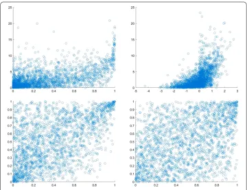
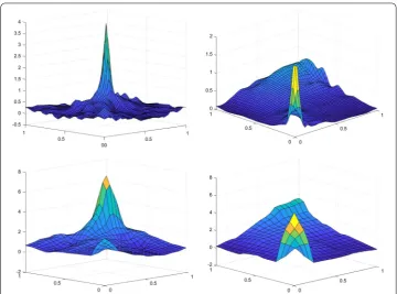
The plots are shown in Figs.1and2. In both figures the scatter plots in the top row show what happens whenF2is exponential with mean 1/3 andF1is eitherB(0.5, 0.7) orN(0, 1). In the bottom row the left one shows the same scatter plot, but the margins are considered asU(0, 1), and the right one shows the pairs of normalized ranks. It is worth mentioning that Fig.1displays scatter plots generated from the Gumbel copula, and Fig.2displays the same ones from the Clayton copula. As the number of observations is increased, the rank–rank plots are more unreadable. It is clear that for a random sample of sizen= 2000 or more, the square in these plots could be completed filled, and all features of distribu-tion had been lost. As a suggesdistribu-tion, we would consider the plots of the empirical copula function of the pairs (Ri/n,Si/n). For the same data as in panel (d, bottom right) in Figs.1 and2, 3d-histograms of the relative frequencies of the pseudo-observations (Ri/n,Si/n) are illustrated in Fig.3. The plots show the relative frequency ofn= 2000 pairs (Ri/n,Si/n) in a 32×32 regular partitions of the unit square for Gumbel (left column) and Clayton (right column) copulas in two parts, full data (top row) and censored data (bottom row) with Kendall’s tauτ= 1/2.

Figure 1Scatter and rank-rank plots for a sample of size 2000 from the Gumbel copula based on censored data withτ= 1/2, once the margins have been transformed toF1andF2. (a, top left):F1=B(0.5, 0.7) and

F2=ε(3); (b, top right):F1=N(0, 1) andF2=ε(3); (c, bottom left):F1=F2=U(0, 1); (d, bottom right): the rank-rank plot for Gumbel copula

levelJare computed as follows:

˜

αJk1k2= 1

n

n

i=1

winI

k1– 1

N < Ri

n ≤

k1

N, k2– 1

N < Si

n ≤

k2

N

for allk1,k2∈ {1, . . . ,N}. Finally, we obtain the wavelet estimators for Gumbel and Clayton copulas (equation (5)) and consider their plots at levelsJ– 1 andJ– 2. The graphs are in Fig.4.

Step 3:We find the average squared error (ASE) calculated for several wavelet copula

estimators, including (5) for different sample sizesn. The results for ASE and the total number of replicationsN= 100 for two different dependence copula parameters and for wavelet and kernel methods are shown in Table1. The ASE criterion is defined as

ASE= 1

N

N

l=1

1

n2 n

j=1 n

i=1

˜

c(l)(ui,vj) –c(ui,vj)

2

,

where˜c(l)denotes an estimator ofcat thelth replication. In this simulation study, we have used Daubechies’s compactly supported wavelet symmlet8 and levelj0= 5.

sim-Figure 2Scatter and rank-rank plots for a sample of size 2000 from the Clayton copula based on censored data withτ= 1/2, once the margins have been transformed toF1andF2. (a, top left):F1=B(0.5, 0.7) and

F2=ε(3); (b, top right):F1=N(0, 1) andF2=ε(3); (c, bottom left):F1=F2=U(0, 1); (d, bottom right): the rank-rank plot for Clayton copula

ulation results show that the wavelet estimator performs better than kernel estimators in terms of AMSE criterion. We can do the same work for some other copula functions like Gaussian, Frank, and Student copulas or for other wavelets such as Haar or Adelson wavelets.

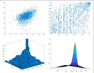
4.2 Real data

Here we present an application of the proposed methodology for the data of [13], where the first observation is censored. The data consist of the indemnity payment (LOSS) and the allocated loss adjustment expense (ALAE) for 1500 general liability claims. The graphical representation of this data is considered in Fig.5. Panels (a) and (b) show logarithm scale of the original data and the rank–rank plot, respectively. In panel (c) the 3D-histogram of Loss (censored) and Alae data is shown based on 16×16 grid. Panel (d) shows the wavelet-based estimator described in Sect.2.

Due to our simulation results, the nonparametric procedure tries to provide a smooth copula estimate, and the wavelet-based estimator is a good estimator under the fact that a considerable copula family is Gumbel. Many authors who used this data in their researches claimed that the best representation of Loss and Alae data is the Gumbel copula.

5 Conclusions

Figure 33d-histograms. (a, top left): Gumbel (full data), (b, top right): Clayton (full data), (c, bottom left): Gumbel (censored data), (d, bottom right): Clayton (censored data)

offer fast computations and easy updating in addition to being easily adapted to the de-sign. We derived an analog of the asymptotic formula of the mean integrated square error in the context of kernel density estimators for censored data, admitting an expansion with distinct squared bias and variance components.

The numerical performance of the proposed linear wavelet density estimators was il-lustrated on simulated datasets. Comparisons between full data and censored data for some different sample sizes were also given. Although using wavelet-based estimator of a copula function is very useful for underlying dependence structure, it does not cover the main conditions of parametric models. In future work we might also consider using a nonlinear wavelet-based copula density estimator for randomly censored data or using for goodness-of-fit testing.

Appendix: Proofs

A.1 Proof of Theorem1

Figure 4Wavelet smoothing ofn= 2000 pairs of normalized ranks from Gumbel (left column) and Clayton (right column). (a, top left) and (b, top right) show wavelet estimators under censored data at levelj=J– 1 withJ= 5 for Gumbel and Clayton copula, respectively. (c, bottom left) and (d, bottom right) show wavelet estimators under censored data at levelj=J– 2 withJ= 5 for Gumbel and Clayton copulas, respectively

Table 1 Computed value for ASE compared between the proposed wavelet estimator in our paper and kernel estimator (defined in lopez(2015)) based on two copulas for various sample sizes

Estimation methods ASE

n= 100 n= 300 n= 500

Wavelet Gumbel (τ= 0.25) 1.07 1.25 1.36

Kernel (h= 0.4) Gumbel (τ= 0.25) 1.32 1.45 1.57

Wavelet Clayton (τ= 0.25) 1.15 1.82 2.02

Kernel (h= 0.4) Clayton (τ= 0.25) 1.37 2.01 2.32

Wavelet Gumbel (τ= 0.75) 6.13 7.32 7.59

Kernel (h= 0.4) Gumbel (τ= 0.75) 6.63 7.66 7.95

Wavelet Clayton (τ= 0.75) 7.20 8.74 9.11

Kernel (h= 0.4) Clayton (τ= 0.75) 7.90 9.31 10.32

Assumption 1 Assume thatE( δ1 1–G)

2

=E(δ1g(T1))2<∞, and assume that there exist i.i.d. random variables (Zi) such thatsup|Win–Wi| ≤BnZi, whereBn=sup|G_1–ˆ–_GG_ˆ |=O(n–1/2) andE[Zi] =E[_1–Gδ1_(Y1i)] <∞.

Also, suppose that the functionφdefined in Sect.2.2ism-differentiable. We define

ξk(Y1i,T2i) =

φj0k

F1n(Y1i),F2n(T2i)

–φj0k

F1(Y1i),F2(T2i)

Figure 5(a, top left): original data on the logarithm scale, (b, top right): rank–rank plot, (c, bottom left): 3D-histogram, panel (d, bottom right): wavelet-based copula density estimate

In addition,α˜j0k–αˆj0k= 1 n

n

i=1Winξk(Y1i,T2i). So we obtain

E

k

(˜αj0k–αˆj0k) 2

=

k

E

1

n

n

i=1

Winξk(Y1i,T2i)

2

=

k

E

1

n

n

i=1

Wiξk(Y1i,T2i) + 1

n

n

i=1

(Win–Wi)ξk(Y1i,T2i)

2

≤2

k

E

1

n

n

i=1

Wiξk(Y1i,T2i)

2

+

k

E

1

n

n

i=1

(Win–Wi)ξk(Y1i,T2i)

2

=: 2(T1+T2).

First, following the proof of Proposition 1 in [14], we obtain a bound forT1:

T1≤ 1

n2

k

i∈I(j,0)∪I1(j,)

EWiξk(Y1i,T2i)

2

+ 1

n2

k

i=l∈I(j,0)∪I1(j, )

Due to the last sentence in Sect.2.1and because of the limit functiong, we get

EWiξk(Y1i,T2i)

2

=gEξk(T1i,T2i)

2 ≤K1E

ξk(T1i,T2i)

2

and also

EWiWlξk(Y1i,T2i)ξk(Y1l,T2l)

=gEξk(T1i,T2i)ξk(T1l,T2l)

≤K1E

ξk(T1i,T2i)ξk(T1l,T2l)

.

Similarly, we haveE(Wi)2=_1–1_G =g≤K1.

Since the support of the scaling function is compact, we finally obtain the bound forT1:

T1≤KK1 1

n22

2j_n2–j₂3jlog(n)

n +KK1

1

n22

2j_n2–j2₂3jlog(n)

n +KK1n

–δ+1

≤K2

2j

n

22jlog(n)

n + 2

–j_log(n)

.

In addition, according to Assumption1, we have

E(Win–Wi)ξk(Y1i,T2i)

2 =E

δ1(Gˆ –G)

(1 –Gˆ)(1 –G)ξk(Y1i,T2i)

2

= (Gˆ –G) 2

(1 –Gˆ)2E

Ziξk(T1i,T2i)

2

≤Kn–1Eξk(T1i,T2i)

2 .

Similarly, the bound for (Win–Wi)ξk(Y1i,T2i) follows:

E(Win–Wi)(Wln–Wl)ξk(Y1i,T2i)ξk(Y1l,T2l)

=(Gˆ –G) 2

(1 –Gˆ)2E

Z2_iξk(T1i,T2i)ξk(T1l,T2l)

≤Kn–1Eξk(T1i,T2i)ξk(T1l,T2l)

.

It remains to find the bound for the last part ofT2:

E(Win–Wi)2=E

δ1(Gˆ –G)

(1 –Gˆ)(1 –G)

2

=(Gˆ –G) 2

(1 –Gˆ)2E(Zi)

2_≤Kn–1_,

where the last equality follows from Assumption1. At the end, the sharper bound forC2 is

T2≤ 1

n2

k

i∈I(j,0)∪I1(j,)

(Gˆ –G)2 (1 –Gˆ)2E

Ziξk(T1i,T2i)

2 + 1 n2 k

i=l∈I(j,0)∪I1(j, )

(Gˆ–G)2 (1 –Gˆ)2E

+Kn–δ22j(Gˆ–G) 2

(1 –Gˆ)2E(Zi) 2

≤KK1n–1 1

n22

2j_n2–j₂3jlog(n)

n +KK1n

–1 1

n22

2j_n2–j2₂3jlog(n)

n +KK1n

–1_n–δ+1

≤K2

2j

n2

22jlog(n)

n + 2

–j_log(n)

.

Therefore with the bounds forT1andT2the proof of Theorem1is complete.

A.2 Proof of the Theorem2

Combining the result of Lemma1and Theorem1and the fact that the error term associ-ated with the use of ranks in the proof of Theorem1is negligible with respect to the usual error term as soon as 2j0_{log(n), the proof is complete.}

Funding Not applicable.

Availability of data and materials

The datasets used and analyzed during the current study are available from the corresponding author on reasonable request.

Competing interests

The authors declare that they have no competing interests.

Authors’ contributions

This work was carried out in collaboration among all authors. All authors read and approved the final manuscript.

Author details

1_{Department of Statistics, Payame Noor University, Tehran, Iran.}2_{Department of Statistics, Payame Noor University,}

Mashhad, Iran. 3_{Faculty of Science, Gonbad Kavous University, Gonbad Kavous, Iran.}

Publisher’s Note

Springer Nature remains neutral with regard to jurisdictional claims in published maps and institutional affiliations.

Received: 6 March 2019 Accepted: 21 June 2019

References

1. Autin, F., Lepennec, E., Tribouley, K.: Thresholding methods to estimate the copula density. J. Multivar. Anal.101, 200–222 (2010).http://doi.org/10.1016/j.jmva.2009.07.009

2. Bouye, E., Durrleman, V., Nikeghbali, A., Riboulet, G., Roncalli, T.: Copulas for finance: a reading guide and some applications. In: Groupe de Recherche Operationelle. Credit Lyonnais, Paris (2000)

3. Bouye, E., Durrleman, V., Nikeghbali, A., Riboulet, G., Roncalli, T.: Copulas for finance—A reading guide and some applications. Social Science Research Network Working Paper Series (2007).https://doi.org/10.2139/ssrn.1032533

4. Butucea, C., Tribouley, K.: Nonparametric homogeneity tests. J. Stat. Plan. Inference136, 597–639 (2006).

http://doi.org/10.1016/j.jspi.2004.08.003

5. Chatrabgoun, O., Parham, G.: Copula density estimation using multiwavelets based on the multiresolution analysis. Commun. Stat., Simul. Comput.45, 3350–3372 (2014)

6. Chatrabgoun, O., Parham, G., Chinipardaz, R.: A Legendre multiwavelets approach to copula density estimation. Stat. Pap.58, 673–690 (2017).http://doi.org/10.1007/s00362-015-0720-0

7. Cherubini, U., Luciano, E., Vecchiato, W.: Copula Methods in Finance. Wiley Finance Series. Wiley, Chichester (2004) 8. Daubechies, I.: Ten Lectures on Wavelets. SIAM, Philadelphia (1992)

9. Deheuvels, P.: La fonction de dépendance empirique et ses propriétés: Un test non paramétrique d’indépendance. Bull. Cl. Sci., Acad. R. Belg. (5)65, 274–292 (1979)

10. Embrechts, P., Kluppelberg, C., Mikosch, T.: Modeling Extremal Events for Insurance and Finance. Springer, Berlin (1997)

11. Fermanian, J.-D., Wegkamp, M.: Time dependent copulas. Preprint (2004).http://doi.org/10.1.1.332.6192

12. Fleming, T.R., Harrington, D.P.: Counting Processes and Survival Analysis. Wiley Series in Probability and Mathematical Statistics: Applied Probability and Statistics. Wiley, New York (1991).http://doi.org/10.1002/9781118150672

13. Frees, E., Valdez, E.A.: Understanding relationships using copulas. N. Am. Actuar. J.2, 1–25 (1998).

http://doi.org/10.1080/10920277.1998.10595667

15. Gribkova, S., Lopez, O.: Non-parametric copula estimation under bivariate censoring. Scand. J. Stat.42, 925–946 (2015).http://doi.org/10.1111/sjos.12144

16. Joe, H.: Multivariate Models and Dependence Concepts. Chapman & Hall, London (1997).

https://doi.org/10.1002/(SICI)1097-0258(19980930)17:18<2154::AID-SIM913>3.0.CO;2-R

17. Li, L.: Non-linear wavelet-based density estimators under random censorship. J. Stat. Plan. Inference117, 35–58 (2003).http://doi.org/10.1016/so378-3758(02)00366-x

18. Meyer, Y.: Wavelets: Algorithms and Applications. SIAM, Philadelphia (1993).http://doi.org/10.1137/1036136

19. Morettin, P.A., Toloi, C.M.C., Chiann, C., de Miranda, J.C.S.: Wavelet smoothed empirical copula estimators. Braz. Rev. Finance8, 263–281 (2010)

20. Nelsen, R.B.: An Introduction to Copulas, 2nd edn. Springer, New York (2006)

21. Patton, A.J.: A review of copula models for economic time series. J. Multivar. Anal.110, 4–18 (2012).

http://doi.org/10.1016/j.jmva.2012.02.021

22. Sklar, A.: Fonctions de répartition àndimensions et leurs marges. Publ. Inst. Stat. Univ. Paris8, 229–231 (1959) 23. Van der Laan, M.J.: Efficient estimation in the bivariate censoring model and repairing NPMLE. Ann. Stat.24(2),

596–627 (1996).http://jstor.org/stable/2242663