A Fast high Order Algorithm for Three dimensional Poisson Equations

2018 International Conference on Computer, Communications and Mechatronics Engineering (CCME 2018) ISBN: 978-1-60595-611-4

A Fast-high Order Algorithm for Three-dimensional Poisson Equations

Wen-jie HE and Na ZHU*

School of Mathematics and Physics, North China Electric Power University Department, Baoding, China

*Corresponding author

Keywords: Three-dimensional Poisson equation, Fast Fourier transform, High-order algorithm.

Abstract. The three-dimensional Poisson equations widely exist in many physical or engineering problems. We proposed a fourth-order fast algorithm for solving the three-dimensional Poisson equation. By the fast Fourier transform, block tridiagonal structure can be generated, and the original problem can be easily decomposed into small independent systems. Fourier operators accelerate the process of solving numerical solutions and greatly reduce the computation time. The accuracy and efficiency of the method are verified by several numerical experiments.

Introduction

In the paper, we consider the following Poisson equation

∆𝑢(𝑥, 𝑦, 𝑧) = −𝑓(𝑥, 𝑦, 𝑧), in Ω (1) with Dirichlet boundary condition

𝑢(𝑥, 𝑦, 𝑧) = 𝑢₀(𝑥, 𝑦, 𝑧), on ∂Ω (2) where is a three-dimensional continuous convex domain and is its boundary. The source function 𝑓(𝑥, 𝑦, 𝑧), the boundary condition 𝑢₀(𝑥, 𝑦, 𝑧) and the exact solution 𝑢(𝑥, 𝑦, 𝑧) are sufficiently smooth and have the necessary continuous partial derivatives up to certain orders.

The three-dimensional Poisson equation is a kind of partial differential equation with wide application range, and its numerical calculation plays a very important role in the numerical simulation of fluid mechanics, heat and mass transfer and so on. In recent years, there has been great interest in algorithms to solve the three-dimensional Poisson equation.

In modern numerical methods, there are many methods to solve Poisson equation, such as Ritz-Galerkin method [1], finite difference method [2], finite volume method and so on [3, 4]. Finite difference method is the earliest and perfect method to solve elliptic problems such as Poisson equation. However, most algorithms are developed for two-dimensional problems.

Fast Fourier transform is a powerful technique for solving three-dimensional Poisson equation. This paper presents a fast algorithm for solving three-dimensional Poisson equations. The large linear system is decomposed into small independent systems by fast Fourier transform, which greatly reduces computation time.

The rest of the paper is organized as follows. In Section 2, a fourth-order finite difference method for the Poisson equation is constructed. Sections 3 proposed a fast algorithm for solving the three-dimensional Poisson equation. Two numerical experiments verify the efficiency of the fast fourth-order algorithm in Section 4. The paper is concluded in Section 5.

The Fourth-Order Finite Difference Method

We consider a fourth-order finite difference method of Equation (1), where Ω is a continuous convex domain in three-dimensional space and ∂Ω is the boundary of the domain. The source function 𝑓(𝑥, 𝑦, 𝑧) is a given continuous function. And 𝑓(𝑥, 𝑦, 𝑧) is assumed to be sufficiently smooth and has the necessary continuous partial derivatives up to certain orders. The boundary condition 𝑢0(𝑥, 𝑦, 𝑧) is suitable. In this paper, a cubic domain 𝛺 = [0, 𝑎] × [0, 𝑏] × [0, 𝑐] is

considered as the solution field. For the primal partition, we discrete Ω _{with uniform mesh sizes} ℎ𝑥=_𝑀+1𝑎 , ℎ𝑦=_𝑁+1𝑏 , ℎ𝑧=_𝐿+1𝑐 in the 𝑥, 𝑦 and 𝑧 coordinate directions respectively. Here 𝑀, 𝑁 and 𝐿

are the number of components in the 𝑥, 𝑦 and 𝑧 coordinate directions. The uniform partition is defined as {𝑥𝑖, 𝑦_𝑗, 𝑧𝑙}_{𝑖,𝑗,𝑙=0}𝑀+1,𝑁+1,𝐿+1 in Ω . Without loss of generality, we consider the case of ℎ = ℎ𝑥=

ℎ𝑦 = ℎ𝑧 since it can be extended second order central difference operator can be written as

𝛿𝑥2𝑢𝑖,𝑗,𝑙=𝑢𝑖+1,𝑗,𝑙− 2𝑢𝑖,𝑗,𝑙+ 𝑢𝑖−1,𝑗,𝑙

ℎ2 ,

𝛿𝑦2𝑢𝑖,𝑗,𝑙=𝑢𝑖,𝑗+1,𝑙− 2𝑢𝑖,𝑗,𝑙+ 𝑢𝑖,𝑗−1,𝑙

ℎ2 ,

𝛿𝑧2𝑢𝑖,𝑗,𝑙=𝑢𝑖,𝑗,𝑙+1− 2𝑢𝑖,𝑗,𝑙+ 𝑢𝑖,𝑗,𝑙−1

ℎ2 ,

where 𝑢_{𝑖,𝑗,𝑙}, 𝑖 = 1,2, ⋯ , 𝑀, 𝑗 = 1,2, ⋯ , 𝑁, 𝑙 = 1,2, ⋯ , 𝐿 refers to the fourth-order finite difference solution of the three-dimensional Poisson equation.

The fourth-order finite difference from can be obtained in the interior of Ω.

(𝛿_𝑥2_{+ 𝛿}

𝑦2 + 𝛿𝑧2)𝑢𝑖,𝑗,𝑙 −

ℎ2

6 (𝛿𝑥2𝛿𝑦2+ ä𝑦2𝛿𝑧2+ 𝛿𝑧2𝛿𝑥2)𝑢𝑖,𝑗,𝑙

= −𝑓 +ℎ₁₂2(𝛿𝑥2+ 𝛿𝑦2+ 𝛿𝑧2)𝑓𝑖,𝑗,𝑙+ 𝑂(ℎ4) (3)

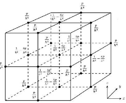
where 𝛿_𝑥2, 𝛿_𝑦2and 𝛿_𝑧2 are standard second order central difference operator and 𝑢_{𝑖,𝑗,𝑙} is the fourth-order finite difference solution of Equation (1). Figure 1 depicts the contributions to the 19-points

stencil in a given axis, where 𝑝 =ℎ

2

Figure 1. The 19-points stencil of fourth-order finite difference method for three-dimensional Poisson equation.

Moreover, Equation (3) can be written in the matrix form

(𝐴𝑀⨂𝐼𝑁⨂𝐼𝐿+ 𝐼𝑀⨂𝐴𝑁⨂𝐼𝐿+ 𝐼𝑀⨂𝐼𝑁⨂𝐴𝐿)𝑈 + 𝑈𝐵

−ℎ2

6 (𝐴𝑀⨂𝐴𝑁⨂𝐼𝐿+ 𝐼𝑀⨂𝐴𝑁⨂𝐴𝐿+ 𝐴𝑀⨂𝐼𝑁⨂𝐴𝐿)𝑈 = −𝐹

+ℎ₁₂2(𝐴𝑀⨂𝐼𝑀⨂𝐼𝐿+ 𝐼𝑀⨂𝐴𝑀⨂𝐼𝐿+ 𝐼𝑀⨂𝐼𝑁⨂𝐴𝐿)𝐹 + 𝐹𝐵. (4)

where

𝐴𝑀= 1

ℎ2𝑡𝑟𝑖𝑑𝑖𝑎𝑔(1, −2,1), 𝐴𝑁= 1

ℎ2𝑡𝑟𝑖𝑑𝑖𝑎𝑔(1, −2,1), 𝐴𝐿= 1

ℎ2𝑡𝑟𝑖𝑑𝑖𝑎𝑔(1, −2,1),

𝑈 = (𝑢_1,1,1, ⋯ , 𝑢_1,1,𝐿, 𝑢_1,2,1, ⋯ , 𝑢_1,2,𝐿, ⋯ , 𝑢_1,𝑁,𝐿, ⋯ , 𝑢_{𝑀,𝑁,𝐿})𝑇, 𝐹 = (𝑓1,1,1, ⋯ , 𝑓1,1,𝐿, 𝑓1,2,1, ⋯ , 𝑓1,2,𝐿, ⋯ , 𝑓1,𝑁,𝐿, ⋯ , 𝑓𝑀,𝑁,𝐿)𝑇,

and the symbol ⨂ represents the Kronecker product. 𝐼𝑀, 𝐼𝑁 and ILare identity matrices, and the

subscripts denote their dimension. 𝐴_𝑀, 𝐴_𝑁 and 𝐴_𝐿 are 𝑀 × 𝑀, 𝑁 × 𝑁 and 𝐿 × 𝐿 tridiagonal metrices respectively. 𝑈_𝐵 and 𝐹_𝐵 contain boundary values subtracted from 𝑈 and 𝐹.

The boundary part consists 18 parts which are related to six surfaces and twelve edges of the

domain, they are

𝑆𝐵𝑡𝑜𝑝, 𝑆𝐵𝑏𝑜𝑡𝑡𝑜𝑚, 𝑆𝐵𝑙𝑒𝑓𝑡, 𝑆𝐵𝑟𝑖𝑔ℎ𝑡, 𝑆𝐵𝑓𝑟𝑜𝑛𝑡, 𝑆𝐵𝑏𝑎𝑐𝑘, 𝐸𝐵𝑡1, 𝐸𝐵𝑡2, 𝐸𝐵𝑡3, 𝐸𝐵𝑡4,

𝐸𝐵𝑐1, 𝐸𝐵𝑐2, 𝐸𝐵𝑐3, 𝐸𝐵𝑐4, 𝐸𝐵𝑏1, 𝐸𝐵𝑏2, 𝐸𝐵𝑏3, 𝐸𝐵𝑏4.

Moreover, the boundary part 𝐹𝐵 includes six parts, and they are

𝐹𝐵𝑡𝑜𝑝, 𝐹𝐵𝑏𝑜𝑡𝑡𝑜𝑚, 𝐹𝐵𝑙𝑒𝑓𝑡, 𝐹𝐵𝑟𝑖𝑔ℎ𝑡, 𝐹𝐵𝑓𝑟𝑜𝑛𝑡, 𝐹𝐵𝑏𝑎𝑐𝑘.

The Fast Algorithm for three-dimensional Poisson Equations

To accelerate the algorithm, we apply the Fourier-sine transformation. For the tridiagonal Toeplitz matrix 𝐴𝑀 and 𝐴𝑁, we have

𝑆𝑀𝐴𝑀𝑆𝑀= 𝛬1= 𝑑𝑖𝑎𝑔(𝜆1, 𝜆2, ⋯ , 𝜆𝑀),

𝜆_𝑖 = −4(𝑀+1)_𝑎 2𝑠𝑖𝑛2 𝑖𝜋

2(𝑀+1), 1 ≤ 𝑖, 𝑗 ≤ 𝑀 (6)

𝑆𝑀 and 𝑆𝑁 are discrete Fourier-sin transformation matrices. 𝑆𝑁 and 𝜇_𝑡, 𝑡 = 1,2, ⋯ , 𝑁 can be

defined similarly as Equation (5) and Equation (6). Multiplying 𝑆𝑀⨂𝑆𝑁⨂𝐼𝐿 on both side of Equation

(4), the following formula can be obtained

(𝛬1⨂𝐼𝑁⨂𝐼𝐿+ 𝐼𝑀⨂𝛬2⨂𝐼𝐿+ 𝐼𝑀⨂𝐼𝑁⨂𝐴𝐿)𝑈̅

−ℎ2

6 (𝛬1⨂𝛬2⨂𝐼𝐿+ 𝐼𝑀⨂𝛬2⨂𝐴𝐿+ 𝛬1⨂𝐼𝑁⨂𝐴𝐿)𝑈̅ + 𝑈̅𝐵= −𝐹̅

+ℎ₁₂2(𝛬1⨂𝐼𝑁⨂𝐼𝐿+ 𝐼𝑀⨂𝛬2⨂𝐼𝐿+ 𝐼𝑀⨂𝐼𝑁⨂𝐴𝐿)𝐹̅ + 𝐹̅𝐵, (7)

where

𝑈̅ = (𝑆𝑀⨂𝑆𝑁⨂𝐼𝐿)𝑈, 𝐹̅ = (𝑆𝑀⨂𝑆𝑁⨂𝐼𝐿)𝐹,

𝑈̅𝐵= (𝑆𝑀⨂𝑆𝑁⨂𝐼𝐿)𝑈, 𝐹̅𝐵= (𝑆𝑀⨂𝑆𝑁⨂𝐼𝐿)𝐹.

Multiplying 𝑆_𝑀⨂𝑆_𝑁⨂𝐼_𝐿 on each part of 𝑈̅_𝐵 , we can obtain

𝑆̅𝐵𝑡𝑜𝑝, 𝑆̅𝐵𝑏𝑜𝑡𝑡𝑜𝑚, 𝑆̅𝐵𝑙𝑒𝑓𝑡, 𝑆̅𝐵𝑟𝑖𝑔ℎ𝑡, 𝑆̅𝐵𝑓𝑟𝑜𝑛𝑡, 𝑆̅𝐵𝑏𝑎𝑐𝑘, 𝐸̅𝐵𝑡1, 𝐸̅𝐵𝑡2, 𝐸̅𝐵𝑡3, 𝐸̅𝐵𝑡4,

𝐸̅_𝐵

𝑐1, 𝐸̅𝐵𝑐2, 𝐸̅𝐵𝑐3, 𝐸̅𝐵𝑐4, 𝐸̅𝐵𝑏1, 𝐸̅𝐵𝑏2, 𝐸̅𝐵𝑏3 and 𝐸̅𝐵𝑏4.

Similarly, multiplying 𝑆𝑀⨂𝑆𝑁⨂𝐼𝐿 each part of 𝐹̅𝐵 , we can obtain

𝐹̅_𝐵

𝑡𝑜𝑝, 𝐹̅𝐵𝑏𝑜𝑡𝑡𝑜𝑚, 𝐹̅𝐵𝑙𝑒𝑓𝑡, 𝐹̅𝐵𝑟𝑖𝑔ℎ𝑡, 𝐹̅𝐵𝑓𝑟𝑜𝑛𝑡, 𝐹̅𝐵𝑏𝑎𝑐𝑘.

Equation (6) is transformed into block-tridiagonal system. Therefore, we can transform the original problem into the following equations

(𝜆𝑖𝐼𝐿+ 𝜇𝑗𝐼𝐿+ 𝐴𝐿) −

ℎ2

6 (𝜆𝑖𝜇𝑗𝐼𝐿+ 𝜇𝑗𝐴𝐿+ 𝜆𝑖𝐴𝐿)𝑈̅𝑖,𝑗,: +𝑈̅𝐵𝑖,𝑗,: = −𝐹̅𝑖,𝑗,:+

ℎ2

12(𝜆𝑖𝐼𝐿+ 𝜇𝑗𝐼𝐿+ 𝐴𝐿)𝐹̅𝑖,𝑗,:+ 𝐹̅𝐵𝑖,𝑗,:, (8)

where 𝑖 = 1,2, ⋯ , 𝑀, 𝑗 = 1,2, ⋯ , 𝑁.

Numerical Experiments

In order to verify the accuracy and reliability of the method presented in this paper, we investigate the following two problems with exact solutions in the three-dimensional unit space Ω = [0,1] × [0,1] × [0,1]. Moreover, both experiments are implemented on MATLAB.

Example 1. Consider the following problem

Δ𝑢(𝑥, 𝑦, 𝑧) = −𝑓(𝑥, 𝑦, 𝑧),

with 𝑓(𝑥, 𝑦, 𝑧) = 0 and the boundary conditions

𝑢(𝑥, 𝑦, 𝑧) = sin(𝜋𝑦) sin(𝜋𝑧) , 𝑥 = 0, 𝑢(𝑥, 𝑦, 𝑧) = 2 sin(𝜋𝑦) sin(𝜋𝑧) , 𝑥 = 1

𝑢(𝑥, 𝑦, 𝑧) = 0, 𝑦, 𝑧 = {0,1}.

, (9)

Here the exact solution is

𝑢(𝑥, 𝑦, 𝑧) =sin(𝜋𝑦) sin(𝜋𝑧)

sinh(𝜋√2) 2 sinh(𝜋√2𝑥) + sinh (π√2(1 − 𝑥)).

Figure 2. Analytical solution with M=64.

Figure 3. Numerical solution with M=64.

Example 2. Consider the following problem

Δ𝑢(𝑥, 𝑦, 𝑧) = −𝑓(𝑥, 𝑦, 𝑧),

𝑓(𝑥, 𝑦, 𝑧) = 3𝜋2_{sin(𝜋𝑥) sin(𝜋𝑦) sin(𝜋𝑧) .} (10)

where the boundary conditions are

𝑢(0, 𝑦, 𝑧) = 𝑢(1, 𝑦, 𝑧) = 0,

𝑢(𝑥, 0, 𝑧) = 𝑢(𝑥, 1, 𝑧) = 0,

𝑢(𝑥, 𝑦, 0) = 𝑢(𝑥, 𝑦, 1) = 0.

Here the exact solution is

𝑢(𝑥, 𝑦, 𝑧) = sin(𝜋𝑥) sin(𝜋𝑦) sin(𝜋𝑧).

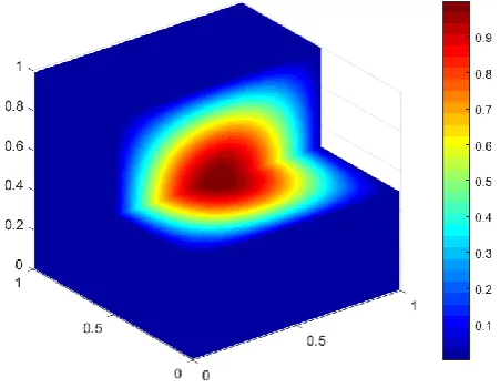
Figure 4. The numerical solution of Equation (10) on the face z=1/2 with 32×32×32 meshes.

Figure 5. The numerical solution of Equation (10) with 32×32×32 meshes.

Figure 6. The numerical solution of Equation (10) with 256×256×256 meshes.

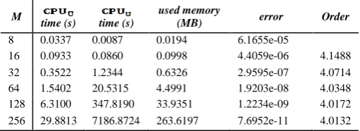
Table 1. CPU time (s), error and convergence order for solving example 2 with different operators.

M

time (s) time (s)

used memory

(MB) error Order

8 0.0337 0.0087 0.0194 6.1655e-05

16 0.0933 0.0860 0.0998 4.4059e-06 4.1488 32 0.3522 1.2344 0.6326 2.9595e-07 4.0714 64 1.5402 20.5315 4.4991 1.9203e-08 4.0348 128 6.3100 347.8190 33.9351 1.2234e-09 4.0172 256 29.8813 7186.8724 263.6197 7.6952e-11 4.0132

Conclusion

In this paper, we proposed a fourth-order fast algorithm for solving the three-dimensional Poisson equation. By fast Fourier transform, the large discrete linear system is decomposed into small independent systems, which greatly save computational memory and time. Several numerical experiments show the feasibility and efficiency of the method.

Acknowledgment

This research was supported by the National Natural Science Foundation of China (No. 11401208), the Natural Science Foundation of Hebei Province (No. A2016502001) and the Fundamental Research Funds for the Central Universities (No. 2018MS129).

References

[1] S. Nintcheu Fata. Semi-analytic treatment of the three-dimensional Poisson equation via a Galerkin BIE method [J]. Journal of Computational and Applied Mathematics, vol. 236, no. 6, pp. 1216-1225, 2011.

[2] S. K. Abd-El-Hafiz, G. A. F. Ismail, B. S. Matit. A numerical technique for the 3-D Poisson equation[J]. Int.j.pure Appl. Math, vol.3, pp. 263-270, 2003.

[3] S. F. Xu, L. Gao, P. W. Zhang. Numerical linear algebra [M]. Beijing: Peking University Press, 2000.

[4] W. Hackbusch. A fast-iterative method for solving Poisson’s equation in a general region[J]. Lecture Notes in Mathematics. vol. 631, 2006.

[5] W. F. Spotz, G. F. Carey. A high-order compact formulation for the 3D Poisson equation [J]. Numerical Methods for Partial Differential Equations, vol. 12, no. 2, pp. 235-243, 1996.

[6] G. F. Dou, Z.Y. Wu, Y.L. Du. The Seven-point Difference Scheme for the Three-dimensional Poisson' s Equation [J]. Chinese Journal of Engineering Geophysics, vol. 6, no. 6, pp. 802-805, 2009.

[7] S. W. Lin, W. M. Zhang, M.Q. Fang, S. Li. A parallel 3D Poisson equation solver based on discrete sine transform [J]. Computer Engineering and Science, vol. 39, no. 8, pp. 1419-1424, 2017.

[8] S. Zhai, X. Feng, Y. He. A family of fourth-order and sixth-order compact difference schemes for the three-dimensional Poisson equation [J]. Journal of Scientific Computing, vol. 54, pp. 97-120, 2013.

[11] P. Mercier, M. Deville. A multidimensional compact higher-order scheme for 3-D Poisson’s equation[J]. Journal of Computational Physics, vol.39, no. 2, pp. 443-455, 1981.

[12] K. Pan, D. He, H. Hu. An extrapolation cascadic multigrid method combined with a fourth-order compact scheme for 3D Poisson equation [J]. Journal of Scientific Computing, vol.70, no.3, pp. 1180-1203, 2017.

[13] J. Wang, W. Zhong, J. Zhang. A general meshsize fourth-order compact difference discretization scheme for 3D Poisson equation [J]. Applied Mathematics and Computation, vol.183, pp. 804-812, 2006.

[14] Y. Ge, Z. Tian, H. Ma. High precision multiple mesh method for solving three dimensional poisson equation[J]. Mathematica Applicata, vol. 19, no. 2, pp. 313-318, 2006.

[15] M. Zhao, Z. Qiao, T. Tang, A fast high order method for electro-magnetic scattering by large open cavities[J], J. Comput. Math, vol. 29, pp. 287-304, 2011.

[16] M. Zhao. A fast high order iterative solver for the electromagnetic scattering by open cavities filled with the inhomogeneous media [J]. Advances in Applied Mathematics & Mechanics, vol.5, no. 2, pp. 235-257, 2013.