R E S E A R C H
Open Access
A smoothing-type algorithm for solving
inequalities under the order induced by a
symmetric cone
Nan Lu
1and Ying Zhang
2** Correspondence: yingzhang@tju. edu.cn
2Department of Mathematics, School of Science, Tianjin University, Tianjin 300072, PR China Full list of author information is available at the end of the article
Abstract
In this article, we consider the numerical method for solving the system of inequalities under the order induced by a symmetric cone with the function
involved being monotone. Based on a perturbed smoothing function, the underlying system of inequalities is reformulated as a system of smooth equations, and a smoothing-type method is proposed to solve it iteratively so that a solution of the system of inequalities is found. By means of the theory of Euclidean Jordan algebras, the algorithm is proved to be well defined, and to be globally convergent under weak assumptions and locally quadratically convergent under suitable assumptions. Preliminary numerical results indicate that the algorithm is effective.
AMS subject classifications:90C33, 65K10.
Keywords:Symmetric cone; Euclidean Jordan algebra, smoothing-type algorithm, global convergence, local quadratic convergence
1 Introduction
LetVbe a finite dimensional vector space over 4 with an inner product 〈·,·〉. If there exists a bilinear transformation fromV×VtoV, denoted by“○,”such that for any x,
y,zÎ V,
x◦y=y◦x; x◦(x2◦y) =x2◦(x◦y); x◦y, z =x, y◦z,
wherex2:=x○x, then (V,○,〈·,·〉) is called a Euclidean Jordan algebra. LetK:= {x2 :
xÎ V}; then Kis a symmetric cone [1]. Thus, Kcould induce a partial order≽: for anyx ÎV, x≽0 means xÎ K. Similarly,x ≻0 meansxÎ intKwhere intKdenotes the interior ofK; andx≼0 means -x≽0.
Let Πk(x) denote the (orthogonal) projection ofxontoK. By Moreau decomposition [2], we can define
x+ : =K(x), x : =x+ −x=K(−x), and |x| :=x++x−= √
x2. (1:1)
The system of inequalities under the order induced by the symmetric cones Kis given by
f(x) 0, (1:2)
where f : V ® V is a transformation (see two transformations:Löwner operator
defined in [3], and relaxation transformation defined in [4]). We assume thatfis con-tinuously differentiable. Recall that a transformationf:V®Vis called to be continu-ously differentiable if the linear operator ∇f(x) :V® Vis continuous at eachx ÎV,
where ∇f(x) satisfyinglimh→0||
f(x+h)−f(x)− ∇f(x)h||
||h|| = 0is the Fréchet derivative
offatx.
When K=n+, (1.2) reduces to the usual system of inequalities over ℜn. In this case, the system of inequalities has been studied extensively because of its various applications in data analysis, set separation problems, computer-aided design pro-blems, image reconstructions, and detection on the feasibility of nonlinear program-ming. Already many iteration methods exist for solving such inequalities; see, for example [5-9]. It is well known that the positive semi-definite matrix cone, the sec-ond-order cone, and the nonnegative orthant cone n+as common symmetric cones have many applications in practice and are studied mostly. Thus, investigation of (1.2) could provide a unified theoretical framework for studying the system of respective inequalities under the order induced by the nonnegative orthant, the sec-ond-order, and the positive semidefinite matrix cones. This is one of the factor that motivated us to investigate (1.2).
Another motivation factor comes from detection on the feasibility of optimization problems. A main method to solve symmetric cone programming problems is the interior point method (IPM, in short). An usual requirement in the IPM is that a feasi-ble interior point of the profeasi-blem is known in advance. In general, however, the diff-culty to find a feasible interior point is equivalent to the one to solve the optimization problem itself. Consider an optimization problem with the constraint given by (1.2) where the interior of the feasible set is nonempty. If an algorithm can solve (1.2) effec-tively, then the same algorithm can be applied to solvef (x) +εe ≼0 to generate an interior point of the solution set of (1.2), whereε>0 is a sufficiently small real number ande is the unique element inVsuch thatx○e=e○x=xholds for allx ÎV(i.e., the identity of V). Thus, a feasible interior point of conic optimization problem could be found in this way.
It is well known that smoothing-type algorithms have been a powerful tool for sol-ving many optimization problems. On one hand, smoothing-type algorithms have been developed to solve symmetric cone complementarity problems (see, for example, [10-14]) and symmetric cone linear programming (see, for example, [15,16]). On the other hand, smoothing-type algorithms have also been developed to solve the system of inequalities under the order induced byn+(see, for example, [17-19]). From these recent studies, a natural question is that how to develop a smoothing-type algorithm to
solve the system of inequalities under the order induced by a symmetric cone. Our
objective of this article is to answer this question.
By the definition of“≼”and the second equality in (1.1), we havef(x)≼0⇔-f(x)ÎK⇔f
(x)-= -f(x)⇔f(x)+=f(x)-+f(x) = 0; that is, the system of inequalities (1.2) is equivalent to
the following system of equations:
Since the transformation involving in (1.3) is non-smooth, the classical Newton methods cannot be directly applied to solve (1.3). In this article, we introduce the smoothing function:
φ(μ, y) =y+y2+ 4μ2e, ∀y∈V, μ∈ . (1:4)
By means of (1.4), we extend a smoothing-type algorithm to solve (1.2). By investi-gating the solvability of the system of Newton equations, we show that the algorithm is well defined. In particular, we show that the algorithm is globally and locally quadra-tically convergent under some assumptions.
The rest of this article is organized as follows. In the next section, we first briefly review some basic concepts on Euclidean Jordan algebras and symmetric cones, and then present some useful results which will be used later. In Section 3, we investigate a smoothing-type algorithm for solving the system of inequalities (1.2) and show that the algorithm is well defined by proving that solvability of the system of Newton equations. In Section 4, we discuss the global and local quadratic convergence of the algorithm. The preliminary numerical results for the system of inequalities under the order induced by the second-order cone are reported in Section 5; some final remarks are provided in Section 6.
2 Preliminaries
2.1 Euclidean Jordan Algebra
In this subsection, we first recall some basic concepts and results over Euclidean Jor-dan algebras. For a comprehensive treatment of JorJor-dan algebras, the reader is referred to [1] by Faraut and Korányi.
Suppose that (V,○, 〈·,·〉) is a Euclidean Jordan algebra which has the identity e. An elementcÎVis called an idempotent ifc○c=c. An idempotentcis primitive if it is nonzero and cannot be expressed by sum of two other nonzero idempotents. For anyx
Î V, letm(x) be the minimal positive integer such that {e,x, x2,..., xm(x)} is linearly dependent. Then, rank of V, denoted by Rank(V), is defined as max{m(x) :xÎV}. A set of primitive idempotents {c1,c2,...,ck} is called a Jordan frame if ci○cj= 0 for any
i,jÎ {1,...,k} withi≠jandkj=1cj=e.
Theorem 2.1(Spectral Decomposition Theorem [1]) Let(V, ○, 〈·,·〉)be a Euclidean Jordan algebra with Rank(V) =r. Then for any xÎ V,there exists a Jordan frame{c1
(x),...,cr(x)}and real numbersl1(x),...,lr (x)such thatx=
r
i=1λi(x)ci(x). The num-bers l1(x),...,lr(x)(with their multiplicities) are uniquely determined by x.
Every li(x)(i Î{1,...,r}) is called an eigenvalue ofx, which is a continuous function with respect to x (see [20]). Define Tr(x) :=ri=1λi(x), where Tr(x) denotes the trace of x. For anyxÎ V, define a linear transformationLx by Lxy =x○y for anyy ÎV. Specially, when Kis the nonnegative orthant conen+, for any x= (x1,...,xn)T , y =
(y1,...,yn)TÎℜn,
Lx= ⎛ ⎜ ⎜ ⎜ ⎝
x1 0 . . . 0 0 x2. . . 0
..
. ... . .. ... 0 0 . . .xn
⎞ ⎟ ⎟ ⎟ ⎠, Lxy=
⎛ ⎜ ⎜ ⎜ ⎝
x1 0 . . . 0 0 x2. . . 0
..
. ... . .. ... 0 0 . . .xn
⎞ ⎟ ⎟ ⎟ ⎠ ⎛ ⎜ ⎜ ⎜ ⎝ y1 y2 .. . yn ⎞ ⎟ ⎟ ⎟ ⎠= ⎛ ⎜ ⎜ ⎜ ⎝
x1y1 x2y2 .. . xnyn
whenKis the second-order coneLn+, for anyx=
x0
¯
x
,y=
y0
¯
y
∈ × n−1,
Lx=
x0 x¯T
¯
x x0I
,Lxy=
x0 x¯T
¯
x x0I y0
¯
y
=
x,y x0y¯+y0x¯
=x◦y;
whenKis the positive semidefinite coneSn+×n, for any X∈Sn+×n
LXY = 1
2(XY+YX) =X◦Y, ∀Y ∈S n×n + ,
For any x,y Î V, xand y operator commute if Lx and Ly commute, i.e.,LxLy =
LyLx. It is well known thatxandy operator commute if and only ifxand yhave their spectral decompositions with respect to a common Jordan frame. We define the inner product 〈·,·〉by 〈x,y〉:= Tr(x○y) for anyx, yÎ V. Thus, the norm on Vinduced by
the inner product is||x||:=√x,x=ri=1(λi(x))2,∀x∈V.
An elementxÎ Vis said to be invertible if there exists ay in the subalgebra gener-ated byxsuch thatx○y=y○x=e, and is written asx-1. Ifx2 =y andxÎK, thenx
can be written asy1/2. GivenxÎ Vwithx=ri=1λi(x)ci(x), where {c1(x),...,cr(x)} is a
Jordan frame and l1(x),...,lr(x) are eigenvalues ofx, then x2=ri=1(λi(x))2ci(x)and |x|=ri=1 λi(x)|ci(x) Furthermore, if li (x) ≥ 0 for all i Î {1,..., r}, then √
x=r
i=1(λi(x)) 1/2
ci(x); and if li (x) >0 for all i Î {1,..., r}, then
x−1=r
i=1(λi(x))− 1
ci(x). More generally, we extend the definition of any real-valued analytic functiong to elements of Euclidean Jordan algebras via their eigenvalues, i.e.,
g(x) :=ri=1g(λi(x))ci(x) where x Î V has the spectral decomposition
x=ri=1λi(x)ci(x).
We recall the Peirce decomposition theorem on the space V. Fix a Jordan frame {c1,...,cr}in a Euclidean Jordan algebraV, fori,jÎ {1,...,r}, define
Vii := {x∈V:x◦ci=x},
Vij := {x∈V:x◦ci= 1
2x=x◦cj}, i=j.
Theorem 2.2 (Peirce decomposition Theorem [1]) The space V is the orthogonal direct sum of spaces Vij(i≤j).Furthermore,
Vij◦Vij⊂Vii+Vjj; Vij◦Vjk⊂Vikifi=k; Vij◦Vkl={0}if{i, j} ∩ {k, l}=∅.
Thus, given a Jordan frame {c1,..., cr}, we can write any element x Î V as
x=ri=1xici+i<jxij, wherexiÎℜandxijÎVij.
2.2 Basic Results
In this subsection, we produce several basic results which will be used in our later analysis.
Proposition 2.1If x≽0,y≽0,and x - y≽0,then√x−√y0.
Proof. The proof is similar to Proposition 8 in [20]; hence we omit it.
suppose that, for any k,ak=r i=1a
k ici+
i<ja
k
ijis the Peirce decomposition of ak with respect to{c1,...,cr}.Then,
(i) if there exists an index iÎ{1,...,r}such thataki → ∞,thenlmax(ak)® ∞and
(ii) if there exists an index iÎ{1,...,r}such thataki → −∞,thenlmin(ak)® -∞,
where lmax(ak)andlmin (ak) denote the largest and the smallest eigenvalues of ak,
respectively.
Proof. For any k, letak=r
j=1λj(ak)ej(ak)be the spectral decomposition ofa
k with
{e1 (ak),...,er(ak)} being a Jordan system. Then, for anyiÎ {1,...,r}, we have
aki||ci||=
r
i=1
akici+ i<j
akij,ci
=ak,ci= r
j=1
λj(ak)ej(ak),ci
≤λmax(ak) r
j=1
ej(ak),ci (sinceej(ak),ci ≥0)
=λmax(ak)e,ci.
(2:1)
SinceLeis positive definite by [1, Proposition III.2.2] andci≠0, it follows〈e,ci〉> 0 and ||ci|| > 0. Thus, from (2.1) we have that lmax(ak) ® ∞when aki → ∞, which
implies that the result (i) holds; Similarly, ak
i||ci||2=
r
j=1λj(ak)ej(ak),ci ≥λmin(ak)rj=1ej(ak),ci=λmin(ak)e,cifor any i Î {1,...,
r}, and hence,lmin(ak)®-∞whenaki → −∞, which implies that the result (ii) holds.
Proposition 2.3Letj(·,·)be defined by(1.4).Then,the following results hold:
(i)j(·,·)is continuously differentiable at any(μ,y)Îℜ++×V with
Dφ(μ,y) (h,v) =v+L−cμ1(4μhe+y◦v),
Where ℜ++:= {a Î ℜ|a > 0}, cμ:=
y2+ 4μ2e, (h, v) Î ℜ × V and Dj(μ, y) denotes the Fréchet derivative of the transformationjat (μ,y).
(ii)j(0, y) = 2y+,andj(0,y)is strong semismoothness at any yÎV.
(iii)j(μ,y) = 0if and only ifμ= 0 and y+= 0.
Proof. (i): It is easy to get the results similar to [11, Lemma 3.1]; hence we omit the proof.
(ii)φ(0,y) =y+y2=y+|y| = 2y
+. In addition, [3, Proposition 3.3] says thaty+ is
strong semismoothness at any y Î V. Thus,j(0,y) is strong semismoothness at anyyÎV.
(iii): It is easy to see that
φ(μ, y) = 0⇔ −y=y2+ 4μ2e ⇔ y2=y2+ 4μ2e, y0.
3 A smoothing Newton algorithm
Let j(·,·) be defined by (1.4). We define a transformationHby
H(z) :=H(μ, x, y) = ⎛
⎝y−f(xμ)−μx φ(μ,y) +μy
⎞
⎠. (3:1)
From Proposition 2.3(iii) it follows that H(μ*, x*,y*) = 0 if and only if μ*= 0, y* = f
(x*) andf(x*)+= 0, i.e.,x* solves the system of inequalities (1.2).
By Proposition 2.3 (i), for any z= (μ, x,y)Îℜ++×V×V, the transformation His
continuously differentiable with
DH(z) (h,u,v) = ⎛
⎝ −hx−D f(hx)u−μu+v hy+ (1 +μ)v+L−1
cμ(4μhe+y◦v
⎞
⎠, (3:2)
where DH(z) denotes the Fréchet derivative of the transformationHat zand (h,u,
v) Î ℜ× V×V. Therefore, we may apply some Newton-type method to solve the smoothing equations H (z) = 0 at each iteration and make μ> 0 and H (z) ®0, so that a solution of (1.2) can be found.
Givenμ >¯ 0, choosegÎ (0, 1), such thatγμ <¯ 1. Define transformations Ψand bas
(z) :=||H(z)||2andβ(z) :=γmin{1, (z)}. (3:3)
Algorithm 3.1(A Smoothing Newton Algorithm)
Step 0 Choose δ Î (0, 1), σ∈
0, 1
2
. Let g be given in the definition of b(·),
μ0=μ¯and (x0, y0) Î V × V be an arbitrary element. Set z0 = (μ0, x0, y0). Set
e0= (μ¯, 0, 0)∈ ×V×Vand k= 0.
Step 1If||H(xk)|| = 0then stop.
Step 2ComputeΔzk= (Δμk,Δxk,Δyk)Îℜ×V×V by
H(zk) +DH(zk) zk=β(zk)e0, (3:4)
where DH(zk)denotes the Fréchet derivative of the transformation H at zk.
Step 3Letlkbe the maximum of the values1,δ,δ2,...such that (zk+λ
k zk)≤[1−2σ(1−γ μ0)λk](zk). (3:5)
Step 4Setzk+1= zk+lkΔzk and k=k+ 1.Go to Step 1.
In order to show that Algorithm 3.1 is well defined, we need to show that the system of Newton equations (3.4) is solvable, and the line search (3.5) will terminate finitely. The latter result can be proved in a similar way as those standard discussions in the literature. Thus, we only need to prove the former result, i.e., the solvability of the sys-tem of Newton equations.
Theorem 3.1 Suppose that f is a continuously differentiable monotone transforma-tion. Then, the system of Newton equations(3.4)is solvable.
Proof. For this purpose, we only need to show thatDH(z) is invertible for allzÎℜ++×
V×V. Suppose thatDH(z)Δz= 0, by (3.4) we have
μ= 0,
− μx−(D f(x) +μI) x+ y= 0,
μy+ (1 +μ) y+Lc−μ1(4μ μe+y◦ y) = 0,
⎫ ⎬
where cμ:=y2+ 4μ2e. Then, from the first and third system of equations in (3.6),
it follows that
[(1 +μ)cμ+y]◦ y=L(1+μ)cμ+y y= 0. (3:7)
By Proposition 2.1 and(1 +μ)2c2
μ−y2= (μ2+ 2μ) (y2+ 4μ2e) + 4μ2e0, we have
that (1 + μ) cμ ≻|y| ≽ -y, and hence, (1 + μ) cμ + y ≻0. Then, by [1, Proposition III.2.2], we know that L(1+μ)cμ+yis positive definite, and so,Δy= 0 holds from (3.7).
Since Df(x) is positive semidefinite from the fact that fis monotone, by the second system of equations in (3.6), we have Δx= 0, which, together with the first system of equations in (3.6), implies that DH(z) is invertible for allzÎℜ++×V×V.
The proof is complete.
Lemma 3.1 Suppose that f is a continuously differentiable monotone transformation and{zk} = {(μk,xk,yk)}⊆ℜ×V×V is a sequence generated by Algorithm 3.1,then we have
(i) The sequences{Ψ(zk)}, {||H(zk)||},and{b(zk)}are monotonically decreasing.
(ii) Define N(γ) :={z∈ +×V×V:μβ¯ (z)≤μ}where the constant gis given in Step 0 of Algorithm 3.1 and the functionb(·)is defined by(3.3),thenzk∈N(γ)for all k.
(iii) The sequence{μk}is monotonically decreasing andμk> 0for all k.
Proof. (i) From (3.5) it is easy to see that the sequence {Ψ(zk)} is monotonically decreasing, and hence, sequences {||H(zk)||} and {b(zk)} are monotonically decreasing.
(ii) We use inductive method to obtain this result. First, it is evident from the choice of the starting point that z0∈N(γ). Second, if we assume that zm= (μm,xm,ym)∈N(γ)for some indexm, then
μm+1− ¯μβ(zm+1) = (1−λm)μm+λmμβ¯ (zm)− ¯μβ(zm+1)
≥(1−λm)μβ¯ (zm) +λmμβ¯ (zm)− ¯μβ(zm+1) =μ¯(β(zm)−β(zm+1))
≥0,
where the first equality follows from the equation in (3.4) and Step 4, the first inequality from the assumption zm∈N(γ), and the last inequality from (i). This shows
thatzm+1∈N(γ), and hence,zk∈N(γ)for allk.
(iii) It follows (3.4) thatμk+1=μk+λk μk= (1−λk)μk+λkμβ¯ (zk). Since μ0 >0,
we can getμk>0 for allkthrough the recursive methods. In addition, by (ii), we have
μk+1= (1−λk)μk+λkμβ¯ (zk)≤(1−λk)μk+λkμk=μk,
4 Convergence of algorithm 3.1
In this section, we discuss the global and local quadratic convergences of Algorithm 3.1. We begin with the following lemma, a generalization of [21, Lemma 4.1], which will be used in our analysis on the boundedness of iterative sequences.
Lemma 4.1Let f be a continuously differentiable monotone function and{uk}⊆V be a sequence satisfying||uk||®∞.Then there exist a subsequence, which we write without loss of generality as {uk},and an index i Î{1,...,r}such that, eitherli(uk)® ∞and fi (uk) is bounded below; or li (uk) ® -∞ and fi (uk) is bounded above, where
uk=r i=1λi(u
k)ei(uk)is the spectral decomposition of uk
, and
f(uk) =ri=1fi(uk)ei(uk) +1≤i<j≤rfij(uk)is the Peirce decomposition of f(uk) with respect to{e1(uk),...,er(uk)}.
Proof. Since ||uk||®∞, passing through a subsequence if necessary, it follows that
J:={i∈ {1,. . .,r}: |λi(uk)| → ∞}.
Define a bounded sequence {vk} withvk=r
i=1(vk)iei(uk)∈V, where
(vk)i=
0, i∈J;
λi(uk), otherwise.
withuk=r i=1λi(u
k
)ei(uk)is the spectral decomposition ofuk. From the definition ofvkand the assumption offbeing monotone, it follows that, for allk,
0≤ uk−vk,f(uk)−f(vk)
=
i∈J
λi(uk)ei(uk), r
i=1
(fi(uk)−fi(vk))ei(uk) + 1≤i<j≤r
(fij(uk)−fij(vk))
=
i∈J
λi(uk)(fi(uk)−fi(vk))||ei(uk)||2.
(4:1)
For any iÎJ, we have |li (uk)|® ∞, and hence, either li(uk)® ∞orli(uk)®-∞. If li (uk)® ∞, then (4.1) shows thatfi (uk) is bounded below by infkfi (vk); ifli(uk) ® -∞, then (4.1) shows that fi (uk) is bounded above by supkfi(vk). Thus, the proof is complete.
Theorem 4.1Suppose that f is a continuously differentiable monotone function, then the sequence {zk}generated by Algorithm 3.1 is bounded and every accumulation point of{xk}is a solution of the system of inequalities (1.2).
Proof. By Lemma 3.1, we have that sequences {μk} and {Ψ(zk)} are nonnegative and monotone decreasing. From (3.1) and (3.3), we have
(zk) =μ2k+||yk−f(xk)−μkxk||2+||φ(μk,yk) +μkyk||2.
Thus, {yk-f(xk) -μkxk} and {j(μk,yk) +μkyk} are bounded. Letg (μk, xk,yk) :=yk- f
(xk) -μkxk, then {g(μk,xk,yk)} is bounded andyk=g(μk,xk,yk) +f(xk) +μkxk. Suppose thatxkhas the spectral decomposition xk=r
i=1λi(xk)ei(xk), then the Peirce
decompo-sition of f(xk) andg(μk,xk,yk) with respect to the Jordan frame {e1(xk),....,er(xk)} are
f(xk) = r
i=1
fi(xk)ei(xk) + 1≤i<j≤r
and
g(μk,xk,yk) = r
i=1
gi(μk,xk,yk)ei(xk) + 1≤i<j≤r
gij(μk,xk,yk) (4:3)
respectively. By (4.2) and (4.3), we have that the Peirce decomposition of yk with respect to {e1(xk),...,er(xk)} is
yk=g(μk,xk,yk) +f(xk) +μkxk
= r
i=1
[gi(μk,xk,yk) +fi(xk) +μkλi(xk)]ei(xk) +
1≤i<j≤r
[gij(μk,xk,yk) +fij(xk)]
:= r
i=1
(yk)iei(xk) + 1≤i<j≤r
(yk)ij.
(4:4)
In the following, we assume that {xk} is unbounded and derive a contradiction. Since
f is a continuously differentiable monotone function, by noticing Lemma 4.1, we can take a subsequence if necessary, without loss of generality denoted by {xk}, and an index i0 Î {1,..., r} such that either λi0(x
k)→ ∞and f i0(x
k)is bounded below; or
λi0(x
k)→ −∞and f i0(x
k)is bounded above. Together with (4.4), it follows that either
λi0(x
k)→ ∞ and (yk)i
0 → ∞; or λi0(x
k)→ −∞ and (yk)i
0→ −∞ with
(yk)i
0=gi0(mk,x
k,yk) + (f(xk))
i0+mk(x
k)i
0. By Proposition 2.2, we further obtain that
either
or
λi0(x
k)→ ∞andλ
max(yk)→ ∞;
λi0(x
k)→ −∞andλ
min(yk)→ −∞.
(4:5)
Suppose that ykhas the spectral decompositionyk=r
i=1λi(yk)ei(yk), then j(μk,yk) +
μkykhas the spectral decomposition
φ(μk,yk) +μkyk= r
i=1
(λi(yk) +
λ2
i(yk) + 4μ2k+μkλi(yk))ei(yk),
hence,
||φ(μk,yk) +μkyk||2= r
i=1
(λi(yk) +
λ2
i(yk) + 4μ2k+μkλi(y
k))2||ei(yk)||2.
(4:6)
We now consider two cases.
Case 1. li0 (xk)® ∞. It follows from (4.5) that lmax(yk)® ∞, which together with
(4.6) implies that
||φ(μk,yk) +μkyk||2≥(
λ2
max(yk) + 4μ2k+ (1 +μk)λmax(yk))2||emax(yk)||2→ ∞,
where emax (yk) denotes the element corresponding to lmax(yk) in the spectral decomposition ofyk.
Case 2.li0(xk)®-∞. It follows from (4.5) thatlmin(yk)® -∞, which together with
(4.6) implies that
||φ(μk,yk) +μkyk||2≥(λmin(yk) +
λ2
min(yk) + 4μ2k+μkλmin(y
k))2||emin(yk)||2
= [4μ2 k/(
λ2
min(yk) + 4μ2k−λmin(y
where emin(yk) denotes the element corresponding tolmin(yk) in the spectral decom-position ofyk. Since4μ2
k/(
λ2
min(yk) + 4μ2k−λmin(yk))→0whenlmin(y
k
)®-∞, so
4μ2k/(
λ2
min(yk) + 4μ2k−λmin(yk)) +μkλmin(yk)→ −∞,
and hence, ||j(μk,yk) +μkyk||2 ®∞ask®∞.
In either case, we get ||j(μk,yk) + μkyk||®∞as k®∞, which contradicts the fact that {j(μk,yk) +μkyk} is bounded. Hence, {xk} is bounded. Since the functionfis con-tinuous, by noticing thatyk=g(μk,xk, yk) +f(xk) +μkxkfor allk, it follows that {yk} is bounded. Therefore, the sequence {(xk, yk)} is bounded.
By Lemma 3.1, we have that sequences {μk}, {||H(zk)||}, and {Ψ(zk)} are nonnegative and monotone decreasing, and hence they are convergent. Denote
lim
k→∞ μk=μ∗, klim→∞||H(z
k)||=H∗, and lim
k→∞(z
k) =∗.
We show thatH* = 0. In the following, we assumeH*≠0 and derive a contradiction. Under this assumption, it is easy to show thatH* > 0,μ*> 0,Ψ* > 0. Sinceμ* > 0 and
the sequence {||H(zk)||} is bounded, we could obtain from the first result that the sequence {(xk, yk)} is bounded. Thus, subsequencing if necessary, we may assume that there exists a point z* = (μ*,x*,y*)Îℜ+×V×Vsuch that limk®∞zk=z*, and hence,
H* = ||H(z*)|| andΨ* =Ψ(z*). Since ||H(z*)|| > 0, soΨ(z*) > 0, from (3.5), it follows that limk®∞lk= 0. Thus, for any sufficiently large k, the stepsizeλˆk:=λk/δdoes not
satisfy the line search criterion (3.5), i.e.,(zk+λˆ
k zk)>[1−2σ(1−γ μ0)λˆk](zk),
which implies that
[(zk+λˆk zk)−(zk)]/λˆk>−2σ(1−γ μ0)(zk).
Sinceμ*> 0, it follows that Ψ(z) is continuously differentiable atz*. Letk®∞, then
the above inequality gives
−2σ(1−γμ¯)(z∗)≤2H(z∗)TDH(z∗) z∗ = 2H(z∗)T(−H(z∗) +β(z∗)e0) =−2H(z∗)TH(z∗) + 2β(z∗)H(z∗)Te0
=−2(z∗) + 2β(z∗)μμ¯ ∗
≤2(−1 +γμ¯)(z∗),
then(−1 +γμ¯)(1−σ)≥0, together withσ ∈
0, 1
2
, it follows thatγμ¯ ≥1, which
contradicts the fact thatγμ <¯ 1. So H* = 0. Thus, by a simple continuity discussion, we obtain that x* is a solution of the system of inequalities (1.2). This shows that the desired result holds.
Now, we discuss the local quadratic convergence of Algorithm 3.1. For this purpose, we need the strong semismoothness of transformation Hwhich can be obtained by Proposition 2.3 (ii). In a similar way as the one in [17, Theorem 3.2], we can obtain the local quadratic convergence of Algorithm 3.1.
Theorem 4.2 Suppose that f is a continuously differentiable monotone function. Let the sequence {zk} be generated by Algorithm 3.1 andz* := (μ*, x*, y*)be an
accumula-tion point of {zk}.If all WÎ ∂H(z*)is nonsingular,where
∂H(z∗) :=conv{lim k→∞DH(u
and conv denotes convex hull,then the whole sequence {zk}converges to z*,and
||zk+1−z∗||=O(||zk−z∗||2), ||H(zk+1)||=O(||H(zk)||2), μk+1=O(μ2k).
5 Numerical experiments
In this section, in order to evaluate the efficiency of Algorithm 3.1, we give some numerical results for solving the system of inequalities under the order induced by the second-order cone (SOCIS, for short) through conducting some numerical experi-ments. All the experiments are done on a PC with CPU of 2.4 GHz and RAM of 2.0 GB, and all codes are written in MATLAB. Throughout the experiments, the para-meters we used are δ= 0.5, s = 0.0001, and g = 0.20. The algorithm is terminated whenever ||H(z)||≤10-6, or the step lengtha ≤10-6, or the number of iteration was over 500. The starting points in the following test problems are randomly chosen from the interval [-1, 1]. In our experiments, the functionHdefined by (3.1) is replaced by
H(z) :=H(μ,x,y) = ⎛
⎝y−f(xμ)−cμx φ(μ,y) +cμy
⎞ ⎠,
where cis a constant. This does not destroy all theoretical results obtained in the previous sections. Denote
Km:={x= (x1,x2)∈ × m−1:x1≥ x2},
then Kmis anm-dimensional second-order cone. First, we test the following problem.
Example 5.1 Consider the system of inequalities(1.4) with f(x) :=Mx+q, and the order induced by the second-order coneK:=Kn1× · · · ×Knm, where M=BBTwith BÎ ℜn× n
being a matrix every of which is randomly chosen from the interval[0, 1]and q
Î ℜn
being a vector every component of which is1.
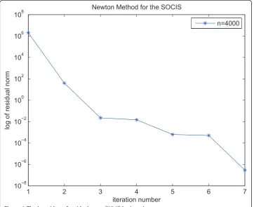
For this example, the test problems are generated with sizes n= 400, 800,..., 4000 and each ni= 10. The random problems of each size are generated 10 times, and thus, we have totally 100 random problems. Table 1 shows the average iteration numbers (iter), the average CPU time (cpu) in seconds, and the average residual norm ||H(z)|| (res) for 10 test problems given in Example 5.1 of each size, for the random initializa-tions, respectively. Figure 1 shows the convergence behavior of one of the largest test problems, i.e.,n= 4000.
Second, we test the following problem, which is taken from [22].
Example 5.2Consider the system of inequalities(1.4)with
f(x) := ⎛ ⎜ ⎜ ⎜ ⎜ ⎜ ⎜ ⎝
24(2x1−x2)3+ exp(x1−x3)−4x4+x5
−12(2x1−x2)3+ 3(3x2+ 5x3)/
1 + (3x2+ 5x3)2−6x4−7x5
−exp(x1−x3) + 5(3x2+ 5x3)/
1 + (3x2+ 5x3)2−3x4+ 5x5 4x1+ 6x2+ 3x3−1
−x1+ 7x2−5x3+ 2
⎞ ⎟ ⎟ ⎟ ⎟ ⎟ ⎟ ⎠ ,
and the order induced by the second-order cone K:=K3×K2.
This problem is tested 20 times for 20 random starting points. The average iteration number is 5.250, the average CPU time is 0.002, and the average residual norm ||H
From the numerical results, it is easy to see that Algorithm 3.1 is effective for the problems has tested. We have also tested some other inequalities, and the perfor-mances of Algorithm 3.1 are similar.
6 Remarks
[image:12.595.117.479.100.236.2]In this article, we proposed a smoothing-type algorithm for solving the system of inequalities under the order induced by the symmetric cone. By means of the theory of Euclidean Jordan algebras, we showed that the system of Newton equations is solvable. Furthermore, we showed that the algorithm is well defined and is globally convergent under weak assumptions. We also investigated the local quadratical convergence of the algorithm. Moreover, the proposed algorithm has no restrictions on the starting point Table 1 Average performances of Algorithm 3.1 for ten problems
n iter cpu res
400 24.500 1.053 1.552e-007
800 29.500 4.365 2.953e-007
1200 22.800 7.194 3.429e-007
1600 24.333 13.580 4.467e-007
2000 12.667 11.038 2.146e-007
2400 15.444 19.891 3.419e-007
2800 15.667 31.102 3.693e-008
3200 12.100 36.105 1.249e-007
3600 14.500 59.270 2.043e-007
4000 16.625 92.832 3.888e-007
1 2 3 4 5 6 7
10−8 10−6 10−4 10−2 100 102 104 106
108 Newton Method for the SOCIS
iteration number
log o
f residual norm
n=4000
[image:12.595.118.481.427.722.2]and solves only one system of equations at each iteration. The preliminary numerical experiments show that the algorithm is effective.
Acknowledgements
This study was partially supported by the National Natural Science Foundation of China (Grant No. 10871144) and the Seed Foundation of Tianjin University (Grant No. 60302023).
Author details
1Department of Mathematics, Xi dian University, XiAn 710071, PR China2Department of Mathematics, School of Science, Tianjin University, Tianjin 300072, PR China
Authors’contributions
YZ conceived the study and participated in its design and coordination. YZ and NL prepared the manuscript initially and performed the numerical experiments. Both of the authors read and approved the final manuscript.
Competing interests
The authors declare that they have no competing interests.
Received: 3 October 2010 Accepted: 16 June 2011 Published: 16 June 2011
References
1. Faraut, J, Korányi, A: Analysis on Symmetric Cones. Oxford Mathematical Monographs, Oxford University Press, New York (1994)
2. Moreau, JJ: Déomposition orthogonale d’un espace hilbertien selon deux cônes mutuellement polaires. C R Acad Sci Paris255, 238–240 (1962)
3. Sun, D, Sun, J: Löwner’s operator and spectral functions in Euclidean Jordan algebras. Math Oper Res.33, 421–445 (2008). doi:10.1287/moor.1070.0300
4. Lu, N, Huang, ZH, Han, J: Properties of a class of nonlinear transformation over euclidean Jordan algebras with applications to complementarity problems. Numer Func Anal Optim.30, 799–821 (2009). doi:10.1080/ 01630560903123304
5. Daniel, JW: Newton’s method for nonlinear inequalities. Numer Math.21, 381–387 (1973). doi:10.1007/BF01436488 6. Macconi, M, Morini, B, Porcelli, M: Trust-region quadratic methods for non-linear systems of mixed equalities and
inequalities. Appl Numer Math.59, 859–876 (2009). doi:10.1016/j.apnum.2008.03.028
7. Mayne, DQ, Polak, E, Heunis, AJ: Solving nonlinear inequalities in a finite number of iterations. J Optim Theory Appl.33, 207–221 (1981). doi:10.1007/BF00935547
8. Morini, B, Porcelli, M: TRESNEI, a Matlab trust-region solver for systems of nonlinear equalities and inequalities. Comput Optim Appl.
9. Sahba, M: On the solution of nonlinear inequalities in a finite number of iterations. Numer Math.46, 229–236 (1985). doi:10.1007/BF01390421
10. Huang, ZH, Hu, SL, Han, J: Global convergence of a smoothing algorithm for symmetric cone complementarity problems with a nonmonotone line search. Sci China Ser A.52, 833–848 (2009)
11. Huang, ZH, Ni, T: Smoothing algorithms for complementarity problems over symmetric cones. Comput Optim Appl.45, 557–579 (2010). doi:10.1007/s10589-008-9180-y
12. Kong, LC, Sun, J, Xiu, NH: A regularized smoothing Newton method for symmetric cone complementarity problems. SIAM J Optim.19, 1028–1047 (2008). doi:10.1137/060676775
13. Liu, XH, Gu, WZ: Smoothing Newton algorithm based on a regularized one-parametric class of smoothing functions for generalized complementarity problems over symmetric cones. J Ind Manag Optim.6, 363–380 (2010)
14. Lu, N, Huang, ZH: Convergence of a non-interior continuation algorithm for the monotone SCCP. Acta Mathematicae Applicatae Sinica (English Series).26, 543–556 (2010). doi:10.1007/s10255-010-0024-z
15. Liu, XH, Huang, ZH: A smoothing Newton algorithm based on a one-parametric class of smoothing functions for linear programming over symmetric cones. Math Meth Oper Res.70, 385–404 (2009). doi:10.1007/s00186-008-0274-1 16. Liu, YJ, Zhang, LW, Wang, YH: Analysis of smoothing method for symmetric conic linear programming. J Appl Math
Comput.22, 133–148 (2006)
17. Huang, ZH, Zhang, Y, Wu, W: A smoothing-type algorithm for solving system of inequalities. J Comput Appl Math.220, 355–363 (2008). doi:10.1016/j.cam.2007.08.024
18. Zhang, Y, Huang, ZH: A nonmonotone smoothing-type algorithm for solving a system of equalities and inequalities. J Comput Appl Math.233, 2312–2321 (2010). doi:10.1016/j.cam.2009.10.016
19. Zhu, JG, Liu, HW, Li, XL: A regularized smoothing-type algorithm for solving a system of inequalities with aP0-function. J Comput Appl Math.233, 2611–2619 (2010). doi:10.1016/j.cam.2009.11.007
20. Gowda, MS, Sznajder, R, Tao, J: SomeP-properties for linear transformations on Euclidean Jordan algebras. Linear Algebra Appl.393, 203–232 (2004)
21. Gowda, MS, Tawhi, MA: Existence and limiting behavior of trajectories associated withP0-equations. Comput Optim Appl.12, 229–251 (1991)
22. Hayashi, S, Yamashita, N, Fukushima, M: A combined smoothing and regularization method for monotone second-order cone complementarity problems. SIAM J Optim.15, 593–615 (2005). doi:10.1137/S1052623403421516
doi:10.1186/1029-242X-2011-4