An Operator Smoothing with ILU(0) for Aggregation based Algebraic Multigrid

2018 3rd International Conference on Computational Modeling, Simulation and Applied Mathematics (CMSAM 2018) ISBN: 978-1-60595-035-8

An Operator Smoothing with ILU(0) for Aggregation-based

Algebraic Multigrid

Jian-ping WU

and Liang SUN

School of Meteorology and Oceanography, National University of Defense Technology, Changsha, China

*Corresponding author

Keywords: Incomplete factorization, Algebraic multigrid, Sparse linear system, Conjugate gradient iteration, Preconditioner.

Abstract. Due to the potential optimal convergence, algebraic multigrid is widely used in solving large sparse linear systems. The aggregation-based version is one of the widely used methods for its cheap cost and easy implementation. But its convergence is often slow compared to other versions. In this paper, a smoothing technique based on incomplete LU factorization without fill-in is presented to the operators on each level. Each operator is approximately factorized, and the derived lower and upper triangular factors are approximately inverted, which are applied to the operator from both sides to improve the diagonal dominance, and then the effectiveness of the smoothing process and the accuracy of the grid transfer operators. The numerical results show that when incorporated into the preconditioned conjugate gradient iteration, the convergence rate is greatly improved, and though the time used for setup is larger, the time used for iteration and the overall time can also be reduced for large-scale systems.

Introduction

Solution of sparse linear systems is the most time-consuming part in many scientific and engineering fields, and with the increasing demand in high resolution simulation, the derived systems are becoming larger and larger. To solve this kind of system efficiently, the multigrid like methods are often used, either as iterations solely, or as preconditioners for Krylov subspace iterations [1].

The effectiveness of multigrid is from the coupling of two processes, the smoothing and the coarse grid correction. The smoothing reduces the error with lower frequencies and the residual corresponding to the remaining error with higher frequencies is transferred to a coarser grid. With the derived residual as the right-hand side, the coarse grid system is solved and its solution is prolonged back to the finer grid, to correct the solution of the original system [2].

Due to potential optimal convergence, multigrid methods attract more and more attention in recent years. Algebraic multigrid methods can achieve similar performance as the traditional geometry versions, without the requirements to know the physical grid or the coordinates in advance, which can be used to solve general sparse linear systems. According to the coarsening process and the construction of the grid transfer operators, algebraic multigrid can be classified into classical and aggregation-based version [2] [3], where the aggregation-based version attracts more attention for its cheap cost and easy implementation. For more details about aggregation-based multigrid methods, we can refer to [4-11].

scheme, each coefficient matrix is approximately factorized, and the derived lower and upper triangular factors are approximately inverted, which are applied to the coefficient matrix from both sides.

Operator Smoothing with ILU(0) for Aggregation-Based Multigrid Method

Aggregation-Based Multigrid Method

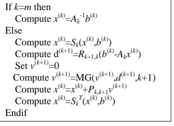
Consider the linear system Ax=b, where A is an n by n positive definite matrix, and b is a vector of dimension n. General multigrid with V-cycle can be described as figure 1[3].

Figure 1. General V-cycle multigrid x(k)=MG(x(k),b(k),k).

In algorithm MG, matrix Sk is a smoothing operator on level k, and SkT is the adjoint of Sk, which assures the positive definiteness of the derived multigrid preconditioner, to apply the preconditioned conjugate gradient iterations. Pk,k+1 is an interpolation operator, to transfer a vector on the k-th level to

the (k+1)-th level, and Rk+1,k is a restriction operator, to transfer a vector on the (k+1)-th level to the

k-th level. In general, we adopt Rk+1,k=Pk,k+1T for symmetric positive cases and Ak+1=Rk+1,k Ak Pk,k+1.

Before applying MG to solve a sparse linear system, the smoother Sk, the interpolation operator

Pk,k+1 and a coaring scheme should be given, and the coarse grid operator Ak+1 should be derived at the

setup first. Any kind of simple iteration can be selected as a smoother. And once the interpolation operator is given, the coarse grid transfer operator can be computed from the finer grid operator. Therefore, the classic algebraic multigrid and aggregation based versions differ mainly in the construction of the grid transfer operator Pk,k+1, and the coarsing scheme.

Assume that matrix Ak is symmetric positive definite, it is corresponding to an undirected graph

Gk=(Vk, Ek), where each vertex in Vk relates to a row/column of Ak, and each edge in Ek relates to a nonzero element of Ak. In aggregation based multigrid algorithm, the vetexes in Vk are classified into different aggregates, with each aggregate corresponding to a vetex in the coaser grid. The classic scheme to construct the tranfer operator is to set Pk,k+1(i, j)=1 if vertex i belongs to the j-th aggregate,

and Pk,k+1(i, j)=0 otherwise.

Operator Smoothing with ILU(0)

To investigate the convergence of multigrid, we usually consider the simplified case of two-level grids, where the iteration matrix can be written as[7]

) )(

)(

( _{k k k,k 1 k}1_{1 k}T_{,k 1 k k}T _k

k I S A I P A P A I S A

T    _ _{ } 

. (1) Therefore, the convergence rate is influenced by two factors.

Firstly, the more accurate Sk approximates the inverse of Ak, the more rapid the convergence rate will be. It is well known that the more diagonally dominant the matrix Ak is, the easier we construct related efficient smoothers, that is, SkAkI is more accurate. Then, the corresponding two-grid iteration will converge more rapidly.

Secondly, we know that when multigrid is used to solve partial differential equations, the stronger the anisotropy is, the less efficient the solver will be. From the point of discrete solution, anisotropy

If k=m then

Compute x(k)=Ak-1b(k)

Else

Compute x(k)=Sk(x(k),b(k))

Compute d(k+1)=Rk+1,k(b(k)-Akx(k))

Set v(k+1)=0

Compute v(k+1)=MG(v(k+1),d(k+1),k+1) Compute x(k)=x(k)+Pk,k+1v(k+1)

Compute x(k)=SkT(x(k),b(k))

relates to differences of off-diagonal elements in the coefficient matrix of the sparse linear system. If the off-diagonal non-zeros are not far different from each other, the more convenient for us to construct an efficient interpolation operator, which is crucial to rapid convergce of the derived multigrid method.

With the above considerations, it is clear that if we can transform Akxk=bk to another linear system

Akxk=bk with Ak approaches the unity I and off-diagonals almost the same in magnitude, the modified multigrid will be more efficient.

In this paper, it is assumed that Ak is symmetric positive and ILU(0)[1][12] is used for the above transformation, then, we have AkLkUk with Uk=LkT, and Lk-1AkLk-TI. In algebraic multigrid method, the coefficient matrix on each level should be given explicitly, thus, we should approximate Lk-1 first.

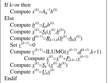
Now, if we denote LkLk-1, and Ak=LkAkLkT, we can apply MG algorithm to Ak recursively, and the modified multigrid algorithm can be described as figure 2, where Sk, Rk, and Pk are similarly defined as Sk, Rk, and Pk respectively, and are all derived from Ak.

From figure 2, we can see that once Lkis derived, the computation can be performed similar to figure 1. The only added operations are the application of Lk and LkT to a vector respectively.

Figure 2. Modified V-cycle multigrid x(k)_=ILUMG(x(k)_,b(k)_,k).

Some Implementation Details in Setup

Now we investigate the computation of Lk and Ak. For Lk is from ILU(0) of Ak, it is suitable to compute

Lk from Lk with the same non-zero structure. Then, if there is a nonzero lk(i,j) in Lk, the corresponding element in Lk is given by

  

 

 

. )

, ( / ) , ( / ) , (

, ),

, ( / 1 ) , (

j i j j l i i l j i l

j i i

i l j

i l

k k k

k k

(2) Assume that matrix Lk is of order nk and it is storedin MSR format[12] to vectors lI and l, where the first nk elements of l are the diagonals one by one, the remaining off-diagonal non-zeros are followed row by row. When i is not larger than nk+1, lI(i) record the position of the first element in the i-th row in vector l. Otherwise, it record the column index of the element l(i). In addition, we store L in CSR format[12] to the vectors lr, lc, and l, with the non-zeros stored in l row by row, the column index of l(k) stored in lc(k), the position of the first element in the i-th row in vector l denoted as lr(i), then the computation is very direct and efficient, and only one traversal of the related vectors is required. The algorithm can be described in detail as figure 3.

To compute Ak, the kernel is the multiplication of two sparse matrices. Assume that it is needed to compute S=AW. Since the i-the row of S can be computed as





 

 

) , ( Adj 1

,*) ( ) , ( ,*)

( ) , ( ,*)

(

i A j n

j

j w j i a j

w j i a i

s

, (3)

If k=m then

Compute x(k)=Ak-1b(k)

Else

Compute b(k)=Lkb (k)

Compute x(k)=Sk(x(k),b(k))

Compute d(k+1)=Rk+1,k(b(k)-Akx(k))

Set v(k+1)=0

Compute v(k+1)=ILUMG(v(k+1),d(k+1),k+1) Compute x(k)=x(k)+Pk,k+1v(k+1)

Compute x(k)=SkT(x(k),b(k))

Compute x(k)=Ukx(k)

where adj(A,i) denotes the column indices of the non-zeros in the i-th row of matrix A. Then, we can compute the vector s(i,*) with sparse data structures.

If matrix A is of order n, we store it in CSR format to the vectors ar, ac, and a, with the non-zeros stored in a row by row, the column index of a(k) stored in ac(k), the position of the first element in the

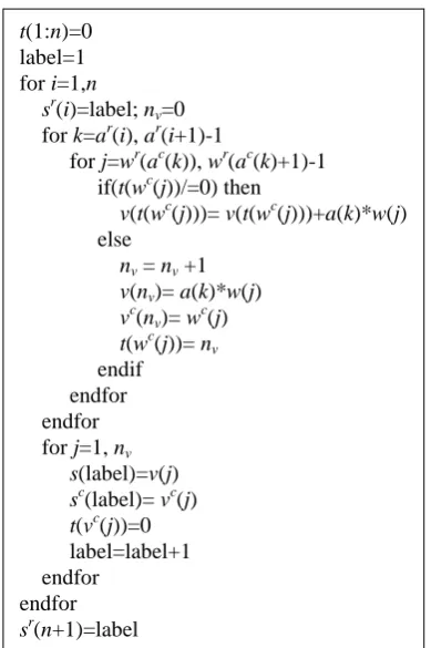
i-th row in vector a denoted as ar(i), and matrix W is stored in the vectors wr, wc, and w similarly, the algorithm to compute S=AW can be described as figure 4. In figure 4, vector t is used to identify whether an element in the current row is already generated. If Sij is generated, it is updated latter when needed. On output, the result matrix S is stored in vectors sr, sc, and s.

Figure 3. Compute ILU(0) inverse of a lower triangular matrix.

Figure 4. Sparse matrix multiplication S =AW in CSR format.

For Ak=LkAkLkT, it can be computed as Bk=LkAk first, and then Ak=BkLkT, where LkT can be stored as

Uk in CSR format, which is transformed from the CSR format of Lk with sparse data structures again. It is clear that we can apply any incomplete factorizations, but we adopt ILU(0) here for two reasons. First when ILU(0) is used, it is cost-effective to compute Lk and Uk from Lk and Uk respectively. Second, for the non-zero pattern of Lk and Uk are similar to that of Ak, then the number of non-zeros in Ak can be controlled in some sense, leading to affordable additional computation costs. When the preconditioned conjugate gradient method is used with the described multigrid as a preconditioner, if the convergence is greatly accelerated, the number of iterations will be largely

label=1 for i=1, nk

lr(i)=label for j=lI(i),lI(i+1)-2

lc(label)=lI(j)

l(label)=-l(j)/l(lI(j))/ l(i) label=label+1

endfor lc(label)=i l(label)=1/l(i) label=label+1 enddo

lr(nk+1)=label

t(1:n)=0 label=1 for i=1,n

sr(i)=label; nv=0

for k=ar(i), ar(i+1)-1

for j=wr(ac(k)), wr(ac(k)+1)-1 if(t(wc(j))/=0) then

v(t(wc(j)))= v(t(wc(j)))+a(k)*w(j) else

nv = nv +1

v(nv)= a(k)*w(j)

vc(nv)= wc(j)

t(wc(j))= nv

endif endfor endfor for j=1, nv

s(label)=v(j) sc(label)= vc(j) t(vc(j))=0 label=label+1 endfor

reduced. Then the overall computation cost will be reduced too, which will be seen from the numerical results from next section.

Numerical Experiments

In this section, we will give some of the test results. All results are derived on a server of Intel(R) Xeon(R) CPU E5-2692 [email protected](cache 30720KB). The operating system is Red Hat Linux 2.6.32-220-TH, and the compiler used is Intel FORTRAN Version 11.1. All the test cases here are symmetric positive, and the preconditioned conjugate gradient is used with multigrid method as a preconditioner. When solving a linear system, the initial guess is the zero vector. For multigrid, we adopt original aggregation version here, with the coarsening scheme presented by Braess [3] and the Jacobi smoothing.

The iteration is stopped once the Euclid norm of the residual vector is reduced by 10-10 in all tests. The time elapsed is recorded in seconds and in all the results, DOF denotes the degree of freedoms, MG and ILUMG denote the aggregation based preconditioners as in figure 1 and 2 respectively.

C(grid) denotes the complexity of grid, that is, the ratio of the number of total vertexes in the

multigrid method divided by the order of the original linear system. C(oper) denotes the complexity of the operator, that is, the ratio of the number of total non-zeros of coefficient matrices on each level divided by the number of non-zeros of the coefficient matrix of the original linear system. Nlev

denotes the number of multigrid levels. Sttime denotes the time elapsed for multigrid setup. Iters and

Cptime denote the number of iterations and the iteration time to solve the linear system respectively.

The linear systems are discretized from Dirichlet boundary value problems of the 2D PDE

, f u y u y x u

x _ 

                       (4) which is defined on region (0,c)(0,c), and the function f and the boundary values are all defined through the assumed true solution u=1. All the linear systems considered here are obtained with finite difference scheme. If we select n+2 points in each direction, and for a continuous function z, denote

z(xi,yj) as zi,j, where

1 , , 1 , 0 , ,   

ih y jh j n

x_{i j} 

, (5) and h=c/(n+1), we can discretize the PDE as

, 2 , 1 , 2 / 1 1 , 2 / 1 , , 1 , 2 / 1 1 , 2 / 1

,j ij i j i j ij ij i j i j ij ij ij

i u  u  u  u  u h f

 _{ } _{ }  _{ } _{ }  (6) j i j i j i j i ij

ij h , 1/2 1/2, , 1/2 1/2, 2              

. (7) In system 1, =1, =0, c=1. In system 2 and 3,

                   ], 1 . 2 , 0 [ & ) 1 , 0 [ , ], 1 . 2 , 0 [ & ) 1 , 0 [ , ), 2 , 1 ( & ) 2 , 1 ( , ], 1 . 2 , 1 ( & ] 1 . 2 , 2 ( , ], 1 . 2 , 1 ( & ] 1 . 2 , 2 ( , 3 3 2 1 1 x y y x y x x y y x                          ]. 1 . 2 , 0 [ & ) 1 , 0 [ , ], 1 . 2 , 0 [ & ) 1 , 0 [ , ), 2 , 1 ( & ) 2 , 1 ( , ], 1 . 2 , 1 ( & ] 1 . 2 , 2 ( , ], 1 . 2 , 1 ( & ] 1 . 2 , 2 ( , 3 3 2 1 1 x y y x y x x y y x       (8) In system 2,

1

1

 _, 3

2210

 _, 5

3310

 _{, (9)}

02 . 0

1

 _,₂ 3_,₃500

In system 3,

x 

1

 _,₂ 2103x_,₃ 3105x

, (11)

x

02 . 0

1

 ,₂ 3x,₃500x. (12)

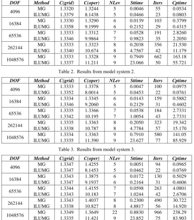
Table 1. Results from model system 1.

DOF Method C(grid) C(oper) NLev Sttime Iters Cptime

4096 MG 1.3320 1.3244 5 0.0046 55 0.0534 ILUMG 1.3379 8.1438 5 0.0466 23 0.0803 16384 MG 1.3330 1.3290 6 0.0139 103 0.3799 ILUMG 1.3358 9.1999 6 0.2152 29 0.4315 65536 MG 1.3333 1.3312 7 0.0528 191 2.8260 ILUMG 1.3346 9.9864 7 0.9823 35 2.2050 262144 MG 1.3333 1.3323 8 0.2038 356 21.530 ILUMG 1.3340 10.674 8 4.7567 42 11.179 1048576 MG 1.3333 1.3328 9 0.7949 662 163.18 ILUMG 1.3337 11.211 9 23.066 50 55.721

Table 2. Results from model system 2.

DOF Method C(grid) C(oper) NLev Sttime Iters Cptime

4096 MG 1.3333 1.3378 5 0.0047 100 0.0975 ILUMG 1.3352 8.0014 5 0.0453 22 0.0761 16384 MG 1.3334 1.3345 6 0.0143 159 0.5882 ILUMG 1.3346 9.2060 6 0.2129 31 0.4602 65536 MG 1.3335 1.3366 7 0.0538 184 2.7331 ILUMG 1.3342 10.195 7 1.0054 43 2.7331 262144 MG 1.3335 1.3363 8 0.2050 323 19.342 ILUMG 1.3338 10.787 8 4.7784 57 15.170 1048576 MG 1.3334 1.3363 9 0.7910 580 141.05 ILUMG 1.3335 11.390 9 23.627 77 85.929

Table 3. Results from model system 3.

DOF Method C(grid) C(oper) NLev Sttime Iters Cptime

4096 MG 1.3347 1.4255 5 0.0051 94 0.0965 ILUMG 1.3347 8.1453 5 0.0462 22 0.0769 16384 MG 1.3343 1.3875 6 0.0172 130 0.5029 ILUMG 1.3347 9.1937 6 0.2164 31 0.4606 65536 MG 1.3344 1.4155 7 0.0598 263 4.0801 ILUMG 1.3343 10.183 7 1.0244 42 2.6706 262144 MG 1.3343 1.4037 8 0.2300 490 30.722 ILUMG 1.3338 10.827 8 4.8817 56 14.920 1048576 MG 1.3349 1.3649 22 0.8830 966 238.29 ILUMG 1.3335 11.421 9 23.852 75 83.903

The test results for solving the three systems with different sizes are listed in table 1 to 3 respectively. From the tables, we can see that, when the problem size is small, ILUMG has no superiority. But ILUMG is less sensitive to the problem size, and with the increase of the size, the convergence rate of ILUMG is faster and faster than MG. For system 2 with discontinuous coefficients, and for system 3 with different strength in different directions, the acceleration is more significant. It is also clear that the convergence rate for any one of the three systems is nearly the same when ILUMG is used, which is very different from MG. When MG is used and the size is unchanged, the number of iterations to solve system 3 is apparently much more than that to system 1 and 2.

Summary

In this paper, we present a technique based on ILU (0) to smooth the coefficient matrices on each level for the aggregation based multigrid methods. The coefficient matrices on each level are factorized with ILU (0) and the triangular factors are approximately inverted with unchanged non-zero patterns. Numerical results show that the modified aggregation based multigrid is superior to the non-modified version. The relatively large operator complexity shows that there are potentials to improve further.

Acknowledgement

This research was financially supported by the National Science Foundation of China (61379022).

References

[1] M. Benzi, Preconditioning techniques for large linear systems: a survey, J. Phys. Comput., 182 (2002) 418-477.

[2] R. D. Falgout, An introduction to algebraic multigrid, Computing In Science & Engineering, 8:6 (2006) 24-33.

[3] C. Wagner, Introduction to algebraic multigrid, Course Notes. University of Heidelberg, 1998/1999; available at: http://www.iwr. uni-heidelberg.de/~Christian.Wagner/.

[4] P. Vanek, J. Mandel, M. Brezina, Algebraic multigrid based on smoothed aggregation for second and fourth order problems, Computing, 56 (1996) 179-196.

[5] M. Brezina, R. Falgout, S. MacLachlan, T. Manteuffel, S. McCormick, J. Ruge, Adaptive smoothed aggregation (SA) multigrid, Siam Review, 47:2 (2005) 317-346.

[6] R. Blaheta, Algebraic multilevel methods with aggregations: An overview, In I. Lirkov, S. Margenov & J. Wasniewski (Eds.), Large-Scale Scientific Computing, 3743 (2006) 3-14.

[7] Y. Notay, Aggregation-based Algebraic Multigrid for Convection-Diffusion Equations. Siam Journal On Scientific Computing, 34:4 (2012) A2288-A2316.

[8] E. Treister, I. Yavneh, On-the-fly adaptive smoothed aggregation multigrid for Markov chains, Siam Journal On Scientific Computing, 33:5 (2011) 2927-2949.

[9] I. Pultarova, Fourier analysis of the aggregation based algebraic multigrid for stochastic matrices, Siam Journal On Matrix Analysis and Applications, 34:4 (2013) 1596-1610.

[10] M. Brezina, A. Doostan, T. Manteuffel, S. McCormick, J. Ruge, Smoothed aggregation algebraic multigrid for stochastic PDE problems with layered materials, Numerical Linear Algebra With Applications, 21:2 (2014) 239-255.

[11] A. Frommer, K. Kahl, S. Krieg, B. Leder, & M. Rottmann, Adaptive Aggregation-Based Domain Decomposition Multigrid for the Lattice Wilson-dirac Operator. Siam Journal on Scientific Computing, 36:4 (2014) A1581-A1608.