Munich Personal RePEc Archive
Coordination failure cycle
Rungcharoenkitkul, Phurichai
December 2005
Online at
https://mpra.ub.uni-muenchen.de/37970/
COORDINATION FAILURE CYCLE
Phurichai Rungcharoenkitkul∗
March, 2012
Abstract
This paper proposes a theory of endogenous fluctuations, grounded on a repeated game with strategic complementarity under incomplete information. The equilibrium is char-acterized by a persistent regime of high activity, where aggregate output tends to expand, followed by a persistent contractionary phase in a recurring cycle. The regime persistence is driven by belief hysteresis, where learning in active regime fuels optimism, propelling an expansion. After an inevitable regime switch, rational persistent pessimism ensues, leading to a prolonged contraction. The equilibrium cycle is unique, stochastic, and converges to a stationary distribution, which characterizes the nature of fluctuations in equilibrium.
Keywords: endogenous cycle, coordination game, learning, global games, hysteresis
JEL Classification: C73, D83, E32
∗E-mail: [email protected] and [email protected]. This paper is based on a chapter of
1
Introduction
The dominant macroeconomic paradigm views aggregate fluctuations as a propagation of exogenous aggregate shocks to fundamentals, but falls short of explaining ‘how’ business cycles arise in the first place. A competing theory may be found in models with multiple rational-expectations equilibria, where changes in expectations can lead to equilibrium shift in a self-fulfilling way, laying the basis for fluctuations unrelated to exogenous shocks.1 However, shifts in expectations still remain unexplained under this approach, leaving multiple equilibria at best a caricature of fluctuations. Moreover, subsequent research has found the existence of multiplicity to be sensitive to small perturbation to payoffs and information structure, which can serve as an equilibrium selection device.2 When a unique equilibrium is selected by such device, strategic complementarity typically ends up playing only a shock propagating role in increasing aggregate volatility, and again there is no room for fluctuations to emerge endogenously.3
This paper proposes a theory of endogenous fluctuations where strategic comple-mentarity plays a central role. The model envisages an economy of large population, whose collective action determines the dynamics of the economy: if a large enough fraction of agents is active, the aggregate output is likely to expand, otherwise fall. An expansion benefits everyone, but particularly those who have been active thus introducing strategic complementarity. With heterogeneous costs of action and incomplete information about others’ costs, each agent must form belief and continuously update her belief as the econ-omy evolves. Type heterogeneity and incomplete information enable a unique strategic equilibrium to be selected, and the equilibrium dynamics is uniquely determined at any given time.
The equilibrium is characterized by a persistent regime of high activity, where the aggregate output keeps rising until some threshold is reached, after which the economy enters a persistent contractionary phase, a regime of low activity. Fluctuations arise as the economy endogenously and perpetually cycles between the two regimes. Regimes are persistent because of belief hysteresis: the event of regime being high tomorrow commands a higher posterior probability if a high regime is observed today, as agents learn that fundamentals must be good enough to justify today’s expansion. Similarly, in a
1
Cooper and John (1988) provide a generalization of the role of strategic complementarity and
multiple equilibria in macroeconomic context, the idea of which dated back to at leastGoodwin(1951) and Keynes’ discussion of animal spirit.
2
Carlsson and van Damme(1993) are a seminal work on equilibrium selection in a coordination game
via an introduction of incomplete information about the game payoffs. The approach proves useful in many macroeconomic applications, and has been extensively explored and generalized. See Morris and
Shin(2003).
3This volatility view of strategic complementarity is generally held by most recent works; for example
Angeletos and Pavan (2007) investigate the sensitivity of unique equilibrium to public information.
Angeletos and La’O (2012) discuss the propagation of shocks to higher-order beliefs, giving rise to
contractionary regime, belief in a low activity equilibrium is reinforced by past observation of low regime. This belief hysteresis results in a persistent play in the selected equilibrium, where an attack on the existing regime never occurs until the expansion has continued for an overly extended period. In the limit, every agent with a nontrivial strategic problem chooses the same action, driving the expansion in a high regime, and the contraction in a low regime.
A number of antecedents are related to this paper. In a seminal work on regime shifts,Chamley(1999) studies a repeated coordination game where a unique equilibrium is also selected and characterized by most players choosing the same action, with occasional regime switches where the players simultaneously switch to the opposite action. The model’s dynamics is driven by an aggregate shock, and regime switches occur when this exogenous shock crosses some thresholds. Chamley’s model therefore views strategic com-plementarity as a propagation mechanism. In contrast, our model produces endogenous cycles in equilibrium, and a qualitatively different dynamic outcome. A key source of departure is that in our model it is the dynamics of aggregate activity that is subject to strategic complementarity in agents’ actions. The aggregate dynamic process has an inherent stabilizing mechanism, as the game payoffs prohibit the aggregate variable from following an explosive path. However, the endogenous dynamics introduces an additional dimension to agents’ learning problem, allowing agents to test their belief about the fundamentals as the state evolves. Under rational learning, this belief moves only with inertia, leading to a lack of steady state. In a high regime, a successively higher output is interpreted as reaffirming the fundamentals to be favorable, encourages agents to continue being active and pushes output higher still, even if the system may in fact edge nearer to its inevitable crash. The reinforcing interactions between learning from past history and the higher-order beliefs allow the effect of regime persistence to dominate, in agents’ calculation, the possibility of an abrupt regime change. The failure to coordinate an early regime switch implies that an expansion can continue prolongedly, forcing a crash only late in a cycle, and similarly for recovery. An endogenous cycle emerges as a result, even if the fundamentals in fact never change.
Our model’s learning dynamics generate a delay in a strategy switch, a property highlighted in many existing works. In the model of bubble in Abreu and Brunnermeier
(2003), rational players find it optimal to ride a bubble for a while, even if they know it must eventually burst, because the incentives to delay selling and time the market make it difficult to synchronize an attack on the bubble until late. In our model, strategic delay to switching actions is also partly incentivized by a short-term gain to production contribution, but crucially the extent of this delay is reinforced by belief hysteresis every time there is an expansion without triggering a crash. The sustained belief hysteresis leads to an outcome of maximal delay, and provides the main impetus in driving the cycle.4 In
Caplin and Leahy(1994) and Chamley and Gale(1994), strategic delay results from the unobservability of other private signals, with an abrupt macro adjustment taking place only when private signals are strong enough for a sufficiently large number of individuals to act, which then causes an information cascade. A form of information cascade also features in our model, as a publicly observed regime switch reveals information about private signals to all players, although in the presence of already maximal delay there is no abrupt change in agents’ optimal strategy after such a switch.
Cycle theory has a long history in economics, but the paradigm is largely regarded as the periphery rather than the core of macroeconomics.5 Firstly, the often deterministic nature of the cycle model gives an excessively sharp prediction, casting doubt on its ability to completely capture phenomenon as complex as the business cycle. Secondly, it is unclear how the model may be empirically tested or fitted to the data. Finally, in many models of this type, cycle is but one possible outcome coexisting along side many others including a steady date, and is therefore far from being a generic description of fluctuations.
Our model’s equilibrium cycle is free of these criticisms. The equilibrium is uniquely selected, predicting fluctuations as a generic phenomenon. At the same time, the equilib-rium cycle is modeled as a Markov process with asymmetric transition probabilities on a closed loop, making the cycle noisy rather than deterministic. The equilibrium outcome converges to a stationary distribution, which, we propose, is a natural equilibrium concept for a model of recurring fluctuations. The equilibrium distribution allows quantitative assessments of welfare and open doors for empirical investigation. In terms of policy implications, we argue that ‘thinking cyclically’ in this way yields new insights that are otherwise not available, while consistent with existing policy wisdom.
The model is set out in Section 2. Section 3 discusses the model’s basic properties and the belief evolution dynamics. The key result of hysteresis and recurring regime switching is derived in Section 4, which implies the existence of cycle. Section 5 provides the conditions ensuring the equilibrium uniqueness. Section 6 explores the quantitative welfare and policy implications of the model, using a simulation exercise, before Section 7 concludes.
a regime switch cannot be immediately followed by another switch. However, this hysteresis effect wanes over time, as the information about the fundamentals become increasingly diffuse in the absence of a regime switch. In our model, agents gain information from the evolution of aggregate variable, which works to sustain the existing regime.
5The cycle approach counts among the early contributors such names as Richard Goodwin, John
Hicks and Nicholas Kaldor. Influential studies on financial crises such asKindleberger and Aliber(2005)
andMinsky(2008) also describe crisis developments as following a recurring cycle pattern. Boldrin and
Woodford (1990) survey the cycle literature and discuss why the approach seems to have fallen out of
2
The Model
2.1
Production technology
Timetis discrete. There is a large population of size normalised ton, and the population set is given by [zt, zt+n], where zt is a stochastic process. There is a single consumption
good, the stock of which is measured in discrete units yt ∈ Y = {0,1, ..., N}. At the
beginning of periodt, agenti∈[zt, zt+n] decides whether to contribute to the production
ofyt, by choosing actionxit ∈ {0,1}denoting inactivity and investment respectively. The
evolution ofyt is determined by joint investment efforts of all agents, R
i∈[zt,zt+n]xitdi, and
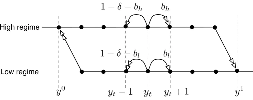
is modelled as a discrete-time birth-and-death process on Y. Specifically, the transition probabilities foryt are given by
Pr
yt+1 =y yt,
Z
i∈[zt,zt+n]
xitdi
=
bt for y=yt+ 1,
δ for y=yt,
1−bt−δ for y=yt−1,
where δ >0 is a constant, and bt is an increasing step function
bt = (
bh for R
i∈[zt,zt+n]xitdi > n−κ,
bl for R
i∈[zt,zt+n]xitdi < n−κ,
(2.1)
where (1−δ)> bh > 1−2δ > bl>0, so that if the number of investing agents exceeds the
threshold n−κ, then the production of an additional unit ofyt is more likely to succeed
than not. It is therefore natural to think of bh and bl as representing the expansionary
and contractionary regimes respectively (high and low regimes, in short). At boundary states N or 0, the probability of yt+1 =yt is δ and that of reflection is 1−δ irrespective
of aggregate investment. Any tie-breaking rule for the case when Ri∈[zt,zt+n]xitdi=n−κ
can be chosen without affecting the key results.
2.2
Agents’ objective function
ytis a public good providing equal utilityu(yt) to all agents for free in each periodt. On
the other hand, contributing to the production ofytis costly. The investment costs differ
across agents, and agent i∈[zt, zt+n] incurs an investment cost ci(yt) if she decides to
invest in period t. In return, each agent who invests at time t will earn an extra private lump-sum gainf at timet+ 1 ifyt+1 =yt+ 1, i.e. if the production at timetis successful
in creating an extra unit of the good. Therefore, choosing to invest amounts to betting that yt will go up next period. The returnf provides private incentive to the production
y
βf b
hβf b
lc
i(
y
)
i
N
{
θ
0
z
tz
t+
n
[image:7.595.145.450.76.254.2]c
zt(
y
)
c
zt+n(
y
)
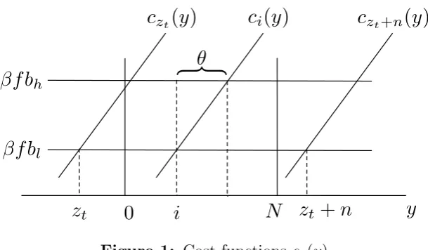
Figure 1: Cost functions ci(y)
The objective function of agenti at time t is the lifetime discounted payoff
Uit =Et ∞ X
s=t
βs−t[u(y
s)−xisci(ys) +fis]
where β is the discount factor and
fit = (
f if yt−yt−1 = 1, and xit−1 = 1
0 otherwise.
Any individual agent’s decision whether to invest clearly depends on the prevailing regime, which in turn depends on other agents’ investment decisions. As will become clear, agents are effectively playing a coordination game.
The cost functions ci(yt) are assumed to take the following linear form
ci(yt) =
βf(bh−bl)
θ (yt−i) +βf bl, i∈[zt, zt+n] (2.2)
where θ > 0. The identity index i serves to identify the cost ranking of agents (i = zt
being the highest-cost agent). The variableztdetermines the aggregate investment cost of
the population, and is therefore a measure of underlying fundamentals. Because the cost functions only depend on the difference yt−i, they satisfy the quasilinearity property,
i.e. any two functions are a horizontal parallel displacement of each other. The fact that i∈[zt, zt+n] also implies a specific correlation structure between the agents’ costs,
amenable to an equilibrium selection mechanism that ensures a unique equilibrium always obtains. Figure 1plots the cost functions ci(y).
2.3
Timing
1. At time t agents hold some identical belief about z∗
t ≡ zt+κ, expressed as a
probability density function ht on a compact interval Zt (ht being zero on R\Zt). The
state yt is observed by everyone.
2. Given such beliefs, all agents choose actions simultaneously to maximise their ex-pected utility. When the equilibrium is unique, the resulting regime is publicly observed. Bayesian rational agents are allowed to revise their beliefs aboutz∗
t. The updated common
belief is denoted by a density ˜ht on an interval ˜Zt. A new stateyt+1 is selected according
to the transition probabilities defined by the regime.
3. After the regime is determined,zt+1 is randomly drawn from a commonly known
uniform transition density p(zt+1|zt), where
p(zt+1|zt) = (
1
2ε if zt+1 ∈[zt−ε, zt+ε]
0 otherwise. (2.3)
In other words, zt is a random walk. A new set of beliefs about zt+1 is generated from
this shock transition rule and the game returns to stage 1, continuing forever thereafter. The parametersθ,κ,nandεare taken to be large relative to 1, so that the dynamics of beliefs can be analysed without being subject to the constraint set by the discreteness of the state space Y. For instance, the assumption implies that yt −θ ≈ yt−1 −θ.
Furthermore, the case of special interest is where ε is small relative to θ, thus limiting the role of exogenous shocks.
As the analysis will show, movements in zt are not the proximate cause of
fluc-tuations in yt. The randomness of zt keeps the posterior belief of zt diffuse and
non-degenerated, which ensures a unique equilibrium selection. Fluctuations in yt are instead
driven by persistence and hysteresis in the agents’ belief, which will be shown to cycle over time. Therefore, fluctuations in this model arise from an endogenous cycle mechanism, and not an amplification of exogenous shocks.
3
Preliminary Analysis
In this section, we first show that the lifetime discounted payoff defined by the stock of goods yt is subject to strategic complementarity, and hence our model is essentially a
series of coordination games with learning over time. There would be multiple equilibria in the complete information case, leading to indeterminate dynamics of yt for some range
of initial conditions. With incomplete information about zt, Bayesian rational agents
form beliefs about the value of zt using all available data, and under some conditions
belief evolution, and the conditions under which a unique switching strategy equilibrium obtains. We then highlight salient features of this belief distribution, central for describing the equilibrium properties in the next section.
3.1
Strategic complementarity
Agent i uses all information available at time t, denoted Ii
t, to form a belief about the
value ofbt, expressed as a perceived probability over{bl, bh}.In view of this, let us define
πit= Pr bt =bh| Iti
(3.1)
and
Eti(bt) = πitbh+ 1−πti
bl.
The value of being agent i at timet,V (Ii
t), is given by
V Iti
= max
x∈{0,1}
n
u(yt)−xci(yt) +β h
Eti(bt)xf + ˜V io
. (3.2)
To understand equation 3.2, note that u(yt) − xci(yt) is simply the period-t payoff
conditional on investment decision x. It is convenient to use x ∈ {0,1} as an indicator function, so that the private return in period t+ 1, conditional on yt+1 =yt+ 1 and x,
is simply given by xf. Thus, the expected private return in period t+ 1 as of time t conditional on x is given by Ei
t(bt)xf. ˜V is a summation of terms involving πti, bh, bl, δ
and the corresponding V Ii
t+1
. When optimising, each agent takes ˜V as a constant, as no single agent can unilaterally affect the evolution of the aggregate stock.
It follows from the functional representation 3.2 then that investment (x = 1) is optimal for agent iat time t if
βf Eti(bt)> ci(yt) (3.3)
which can be reduced to
πti =
yt−i
θ (3.4)
That is, agent iwill invest at time t if she believes the probability of a high regime is sufficiently high. But this probability πi
t is higher if and only if the underlying set
of strategy profiles assigns a larger number of agents to the investment strategy, as agents know the rule determining the regime (equation 2.1). The payoff in each period is therefore subject to strategic complementarity; the return to investment is increasing in the number of opponents who are investing.
a dominant strategy for agent i if ci(yt) < βf bl, i.e. if yt−i < 0. Similarly x = 0 is a
dominant strategy if ci(yt)> βf bh, i.e. ifyt−i > θ. Therefore any agent i∈[zt, zt+n]
does not have a dominant strategy if and only ifyt∈[i, i+θ]. Equivalently, for any fixed
yt, the set of agents without a dominant strategy is given by [yt−θ, yt].
If agent i = z∗
t ≡ zt+κ has a dominant strategy to invest, all other agents with
lower costs also invest, and the regime is guaranteed to be high. When agent z∗
t does
not have a dominant strategy, iterated elimination of dominated strategies can identify a unique switching equilibrium, under which there exists a threshold agent i∗ such that
all i > i∗ invest, while the rest remain inactive. In this equilibrium, a high regime is
guaranteed if z∗
t > i∗, thus agent zt∗ may be referred to as the decisive agent.
Adelay to a regime switch occurs when a large fraction of agents in the strategically nontrivial set [yt−θ, yt] remains invested in equilibrium as long as the regime is high (and
inactive when the regime is low). Thus, there is a greater delay in high regime if i∗ lies
closer to the lower bound of the interval, yt− θ (and in low regime if i∗ is closer to
yt). Longer delay means the prevailing regime has a reinforcing effect to sustain itself in
equilibrium, creating a history-dependent strategy, a property one may call hysteresis.
3.2
Learning and belief evolution
Each stage of the game can be described in more details as follow:
3.2.1 Stage 1: Initial beliefs
Since the same law of evolution is used by all agents for updating purposes, the class of homogeneous beliefs is stationary. In solving the model, it therefore proves convenient to specify some common initial belief. An obvious choice is the shock transition rule, because it is exactly the belief held immediately after a regime switch, which reveals momentarily the true value of zt. Thus, if the value of z∗0 is publicly known at time 1,
then the common belief is that
z1∗ is uniformly distributed on [z0∗−ε, z0∗+ε].
This belief serves as a convenient starting point to compute the general stationary class of homogeneous beliefs in equilibrium.6
6The class of homogeneous beliefs may additionally be dynamically stable under some technical
conditions, as successive learning gradually eliminates any initial belief heterogeneity. Provided that agents’ beliefs ofz∗have the same mean and are distributed over the same support, their belief densities
3.2.2 Stage 2: Equilibrium play
Equilibrium uniqueness is an essential prerequisite for our analysis, as the measurability of the strategy profile with respect to z∗
t is needed for the laws of motion for beliefs to
be well-defined. The sufficient and necessary condition for there to be a unique Bayesian Nash equilibrium surviving iterated elimination of dominated strategies is established by Carlsson and van Damme (1993) in the context of static global game analysis. By a direct application of the global game argument, there is a unique equilibrium in the present model if and only if for all t there exists a unique solutioni∗
t to the equation
Pr [zt∗ > i∗t| It]≡H¯t(i∗t) =
yt−i∗t
θ , (3.5)
where ¯Ht(i) is 1−c.d.f. of belief,
¯ Ht(i)≡
Z supZt
z=i
ht(z)dz. (3.6)
The unique solution, if one exists, corresponds exactly to the unique switching equi-librium, where every agent i < i∗
t chooses x = 0, and every i > i∗t chooses x = 1.7
Note that although there is no heterogeneity in the information set per se, it is the heterogeneous assessments of z∗
t relative toi that results in the applicability of iterated
dominance argument. The details of conditions ensuring a unique solution to equation
3.5 are deferred to section 5.
The existence of at least one dominance region is critical for iterated dominance argument, and is easy to verify in this case. Suppose that the equilibrium has been unique, and the regime switches from high to low at the end of time t. Since z∗
t ∈[infZt, i∗t], the
lower bound for common belief support at timet+ 1 is given by infZt−ε. Note that we
must have infZt < yt−θ (as infZt > yt−θ would imply i∗t =yt−θ <infZt ≤z∗ and
there cannot be a regime switch at time t, a contradiction). It follows that
infZt+1 = infZt−ε
< yt−θ−ε
≈ yt+1−θ−ε
< yt+1−θ
so that there exists a dominance region for a low regime; the decisive agent does not invest as a dominant strategy with some probability. As ε is large relative to 1, this region continues to exist throughout the regime. An analogous argument follows when the regime switches from low to high.
3.2.3 Stage 3: Learning via truncation and transition
At the end of the second stage, provided there exists a unique equilibrium and no regime switch takes place, agents learn that the value of z∗
t must be consistent with the
equilibrium regime and the current state yt. In particular, learning leads to a one-sided
truncation of ht. As before, since the model is symmetric with respect to the regimes, it
suffices to only consider a high regime as the initial condition. The updated distribution is defined by the density ˜ht where
˜
ht(z∗) =
ht(z∗) if infZt≥i∗t,
ht(z∗)
RsupZt z=i∗
t
ht(z)dz otherwise,
= ht(z
∗) RsupZt
z=max{i∗
t,infZt}ht(z)dz
, (3.7)
which is non-zero for z∗ ∈Z˜
t ≡[max{i∗t,infZt},supZt]. A truncation always gives rise
to a nondegenerate interval ˜Z, as ˜Z being empty or a singleton would imply i∗
t ≥supZt,
i.e. i∗
t ≥ zt∗ which violates the assumption that there has not been a regime switch. On
the other hand, if there is a regime switch, say from high to low, at datetthen a learning truncation uses the complementary normalisation, i.e.
˜
ht(z∗) =
ht(z∗) Ri∗
t
z=infZtht(z)dz
(3.8)
for z∗ ∈Z˜
t≡[infZt, i∗t].
Following a shock transition in stage 3, the common belief at timet+ 1 is updated using the shock transition probabilities. Specifically, ht+1 and Zt+1 are given by
ht+1(z∗) =
Z z∗+ε
z=z∗−ε
p(z∗|z) ˜ht(z)dz
= 1
2ε
Z z∗+ε
z=z∗−ε
˜
ht(z)dz, (3.9)
which is positive for
z∗ ∈Zt+1 = [max{i∗t,infZt} −ε,supZt+ε].
Stage 1 can then be repeated.
3.3
Properties of belief distribution
This section establishes the core properties of ht that are needed for the analysis of
stated otherwise, the regime is assumed to be high initially.
First, we define the notion that a density is single-peaked or unimodal, using the following standard definition (the proof for equivalence of each condition is trivial and is omitted). As will be shown, unimodality is an equilibrium property of the belief distribution.
Definition 1. ht(z∗) is ‘unimodal’ if one of the following equivalent conditions holds
(1) ht is decreasing in |z∗−arg maxht(z∗)|, i.e. it always declines away from its
unique peak, or
(2) as z∗ increases, the derivative h′
t(z∗) changes sign (from positive to negative)
at most once, or
(3) there existsz0 such that H¯
t(z∗) is concave for all z∗ < z0 and convex otherwise.
Agents only learn from the outcome of equilibrium play when the initial information about the fundamental is sufficiently vague. For example, in the few periods immediately after a regime switch, the information about the fundamental is already very precise that an ex post equilibrium outcome is unlikely to convey any useful additional information. The following result states that in any period there can be learning if and only if the equilibrium play is not a corner solution. This result will play a useful role in ensuring equilibrium uniqueness later (see the end of section 5.1).
Claim 1. Suppose that the regime is high and that there is a unique equilibrium in period t. The equilibrium exhibits a strictly maximum delay in period t, i.e. i∗
t =yt−θ, if and
only if infZt ≥yt−θ. Furthermore, there is a maximum delay if and only if there is no
learning update (or truncation) in that period.
Proof. See appendix.
Let us now investigate the properties of the shock transition rule. Consider these properties in the context of a pure shock transition, namely when there is no learning truncation in the same period. Under a pure transition, we have ˜ht =ht, and hence
ht+1(z∗) =
1 2ε
Z z∗+ε
z=z∗−ε
ht(z)dz. (3.10)
In other words,ht+1(z∗) is an average ofhton the interval [z∗−ε, z∗+ε]. That the shock
transition rule preserves the symmetry of ht follows immediately from the symmetry of
p(.|.). It is also trivial that the expected value of z∗
t+1 is the same as that of zt∗. The
first important property of the transition mapping is that it leads to a belief of greater ‘riskiness’, as made precise in the next result.
Lemma 1. If ht+1 is a shock transition map of ht, then ht second-order stochastically
Proof. See appendix.
A necessary condition for unimodaltity to be an equilibrium property is the following result.
Claim 2. The unimodality property of a density ht is preserved by the shock transition
rule.
Proof. See appendix.
The last result regarding the shock transition rule underpins the uniqueness result to be obtained later.
Lemma 2. Suppose that ht is unimodal with a unique mode imt , then under a pure
transition mapping,
(1) H¯t crosses H¯t+1 at some point(s) itc on the interval [imt −ε, imt +ε],
(2) if ht is concave on [imt −2ε, imt + 2ε], then there is a unique crossing point ict.
Proof. See appendix.
The concavity requirement is only a sufficient condition for there to be a single crossing between ¯Ht and ¯Ht+1. The following result establishes a more general link
between the single crossing of the cumulative and the density.
Claim 3. On Zt+1\ {infZt+1,supZt+1}, H¯t+1 crosses H¯t once if and only if ht+1 crosses
ht twice.
Proof. See appendix.
Next we turn to investigate the effects of truncations on unimodality property.
Claim 4. If ht is unimodal, then ˜ht is also unimodal, regardless of whether there is a
regime switch at date t. Furthermore, arg max ˜ht(z∗) ≥ arg maxht(z∗), with equality if
and only if i∗
t ≤arg maxht(z∗).
Proof. See appendix.
Claims 2 and 4 together suggest that if ht is unimodal then ht+1 is also
uni-modal. This fact implies that if the common belief is initially given by a unimodal distribution, then it remains unimodal in all periods, and for any t, ¯Ht(i) is concave
for i < arg maxht(z∗), and convex otherwise. To justify the unimodality assumption as
an equilibrium property, it is sufficient to assume that agents’ belief in the first period of the game is a unimodal distribution. Even if agents initially hold a non-unimodal belief in the first period, a sufficiently large number of pure shock transitions will lead to a convergence to a unimodal distribution by the central limit theorem (see section4.1
When there is a truncation in period t, equation 3.7 implies that ˜ht ≥ ht on ˜Zt,
with equality only at the points where ht = 0. Note also that inf ˜Zt = i∗t > infZt and
sup ˜Zt = supZt. The next result readily follows.
Claim 5. A left-sidedly truncated distribution first-order stochastically dominates the original version. For example, if the regime is high and i∗
t >infZt, then
Z supZt
z=z1
˜
ht(z)dz ≥
Z supZt
z=z1
ht(z)dz ∀z1 ∈Zt,
with equality if and only if z1 ∈(−∞,infZ
t]∪[supZt,∞).
Claim5captures the basic effect of a learning truncation; in the absence of a regime switch, agents update their beliefs that the fundamental is conducive to the prevailing regime. If the fundamental zt is fixed (but not observed), this truncation effect leads to
a greater delay and hysteresis next period (see Rungcharoenkitkul(2006)). Here, agents can choose actions only after the fundamental has randomly moved, but the next result states that the effect of learning truncation in terms of delay still holds.
Lemma 3. Provided the equilibrium is unique in all periods, a truncation in period t leads to greater delay in period t+ 1, ceteris paribus.
Proof. See appendix.
Lemma3essentially says that the hysteresis effect of a learning truncation survives the smoothing effect of transition. An immediate corollary is that a larger truncation would lead to a correspondingly larger delay. We finish with the last result on the effect of truncations on the mode of the distribution.
Claim 6. Left (right) truncations cannot lower (increase) the mode of the belief density, ceteris paribus. Specifically, if a truncation (say from the left) implies i∗
t < imt+1−ε, then
the truncation does not affect the mode, i.e. im
t+1 is equal to that yielded from a pure
transition of ht.
Proof. See appendix.
4
Regime Switching and Hysteresis
This section focuses on analyzing the equilibrium hysteresis properties, with equilibrium uniqueness assumed as a working hypothesis. The uniqueness conditions and its verifica-tion will be the issue of the next secverifica-tion.
Due to stochasticz∗
t, the belief evolution is not perfectly coupled with theytprocess,
consequence, the exact degree of hysteresis will depend on both (1) the quantitative impact of truncations (relative toyt dynamics) on the equilibrium, and (2) the frequency
of learning updates. In a high regime for instance, a rising yt will tend to raise i∗t
if either learning updates are infrequent, or learning truncations only increase ¯Ht(i)
marginally. Calculating the net hysteresis effect completely would require a computation of an equilibrium outcome in every possible realisation of two dependent time series, yt
and the corresponding beliefs, a seemingly complicated task.
It is helpful to ask a far simpler question; what is the minimum level of hysteresis, taken across all possible realisations of the stochastics, that can be supported without violating the learning procedure? In other words, for a givenyt, what is the largest value
of i∗
t that could be justified by some history? We attempt to answer these questions by
considering two stages of learning separately.
4.1
The first truncation
In the presence of hysteresis effects, a regime switch from low to high releases a strong public signal to all agents that the fundamental has to be good enough to force such a switch given agents’ prior decisions to delay, which collectively favored the old regime. Given a renewed high optimism, agents with a nondominant strategy may choose to invest with probability one for a number of periods, i.e. the equilibrium is a corner solution of maximum hysteresis for a certain length of time. Eventually however, the beliefs will be sufficiently diffuse that the equilibrium becomes an interior solution again. The date at which such an interior solution appears for the first time following a regime switch is called the period of first truncation. That is, the periods preceding the first truncation only involve pure shock transitions.
In the first date of truncation, the common belief distribution is exceptionally tractable. The assumption that ε is small relative to θ implies that there is a large number of pure shock transitions between regime switches, the accumulative effect of which can be represented as a sum of independent random variables. Irrespective of the initial belief which may be intractable in general, the central limit theorem can be invoked to obtain a limiting distribution of z∗
t, namely a normal distribution.
fundamental (in the sense that the set of potential values of the fundamental is large), the lower the probability that they will assign to a regime switch. Thus if the fundamental has not been observed over a long period of time so that agents are very uncertain about its value, then one may expect agents not to act too aggressively in favour of a regime switch in the first period of truncation. We now seek to confirm this intuition analytically, and thereby characterise the minimum level of hysteresis in the period of first truncation. Suppose that there is a regime switch from low to high in period t = −1, and let all agents hold the same belief in period t = 0 that z∗
0 is a random variable distributed
nondegenerately on the interval Z0 ≡[infZ0,supZ0] with finite mean and variance,
µ0 ≡ Z
z∈Z0
zh0(z)dz
σ02 ≡
Z
z∈Z0
(z−µ0)2h0(z)dz.
The following conjectures about the initial belief are assumed, and need to be verified as part of the equilibrium properties.
Conjecture 1. |Z0| ≡supZ0−infZ0 is small relative to θ.
Conjecture 2. 0≤ σ02
ε2 <∞.
Conjecture 3. There exists a constant γ ∈ (0,1] independent of θ and ε such that infZ0−y0+θ=γθ.
Conjectures 1 and 2 place a limit on the fuzziness of the initial belief. Conjecture
3 requires that the equilibrium play in period t = −1 must not be degenerate in favour of a regime switch. To see this, note that the existence of γ specified in conjecture 3
implies that infZ0 is bounded away fromy0−θ. Since infZ0 =i∗−1−ε, the conjecture is
effectivelyi∗
−1 > y−1−θ+ε. The condition holds in the presence of some hysteresis effects
in equilibrium, as then i∗
−1 would be close to y−1. These conjectures will be verified as
being satisfied in equilibrium after proposition 2 is proved below.
After t periods, provided there is no truncation, we have infZt = infZ0 −tε.
Let the first period of truncation be denoted by t1, i.e. t1 is the lowest t such that
infZt = infZ0 −tε < yt − θ. The first result expresses t1 in terms of the primitive
parameters.
Claim 7. Suppose that conjecture 3 holds. As ε becomes large relative to 1, t1 is
approximately given by
t1 ≃
γθ ε . Proof. By definition,
i.e. there is some small constant c1 < ε such that
t1ε = infZ0−yt1 +θ+c
1
t1ε = infZ0−y0 +θ−(yt1 −y0) +c
1
Since yt −y0 ∈ [−t, t], let us write yt − y0 = α1t where α1 ∈ [−1,1]. Hence, using
conjecture3, we have
t1ε = γθ−α1t+c1
t1 =
γθ+c1
ε+α1
≃ γθ
ε
as γθ is large relative to ε and ε is large relative to 1.
Consider the effect of pure transitions. Abstracting from truncations, and again viewing z∗
t as a random walk,zt∗ can be written as
zt∗ =z0∗+ t X
τ=1
Xτ
where each Xτ is an i.i.d random variable uniformly distributed on [−ε, ε]. It follows
from the uniform transition density that
E(Xτ) = 0
V ar(Xτ) =
ε2
3.
Therefore z∗
t is a sum of independent random variables, with
E(zt∗) = µ0
V ar(zt∗) = σ20+
tε2
3 .
A limiting case of interest is where there are a large number of pure transitions before there is the first truncation. By the central limit theorem, for large t we have
zt∗ →N
µ0, σ02+
tε2
3
so that after a large number of pure transitions,
ht(z∗)≃
1
p
2π(σ2
0 +tε2/3)
exp
"
− (z
∗−µ
0)2
2 (σ2
0+tε2/3)
#
Assume for the moment that a unique equilibrium is always ensured. Lemma 1
implies that there exists an interior equilibrium solution for the first time in the period of first truncation, i.e. at datet1. Our present objective is to determinei∗t1. As ¯Ht1(i) is not available in closed form, the strategy is to obtain an asymptotic approximation for i∗
t1.
Given that the regime is high, the unique interior equilibrium in period t1 is determined
by the intersection between (yt1 −i)/θ and the concave region of ¯Ht1(i). One strategy is then to derive an upper bound for i∗
t1 by constructing a tractable auxiliary ¯H
+
t1 (i) that lies below ¯Ht1(i) on the concave region. This procedure is followed in the proof of the next proposition.
Proposition 1. Let t1 be the first period of truncation, and assume σ20/ε2 < ∞ as in
conjecture 2. Then
lim
t1→∞
i∗t1 =yt1 −θ.
Proof. Consider a point i1 =yt1 −θ+α2, for some smallα2 >0. Ati1 and periodt1, we have from equation 4.1,
ht1(i1)≃
1
p
2π(σ2
0 +t1ε2/3)
exp
"
−(yt1 −θ+α2−µ0)
2
2 (σ2
0 +t1ε2/3)
#
(4.2)
Using identical representations used in the proof of claim7, we can write yt1 =y0+α1t1 for some α1 ∈[−1,1], and µ0−y0+θ≃γθ, as µ0−minz0∗ is of order smaller than θ by
conjecture1. Then, using claim 7, we have
yt1 −θ+α2−µ0 = −(µ0−y0+θ) +α1t1+α2
= −γθ+ α1γθ ε +α2
≃ γθhα1 ε −1
i
≃ −γθ.
Using this equation and claim 7 again, equation4.2 can be written as
ht1(i1) ≃
1
p
2π(σ2
0+t1ε2/3)
exp
"
− (−γθ)
2
2 (σ2
0+t1ε2/3)
#
= p 1
2π(σ2
0+γθε/3)
exp
− 3
γθ ε
23σ20
ε2 ε γθ + 1
. (4.3)
Thus, sinceσ2
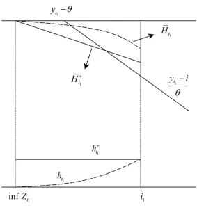
0/ε2 <∞,ht1(i1)→0 exponentially fast as γθ/ε→ ∞. Let us define an auxiliary function h+t1 on [infZt1, i1] as
1
inf
Z
ti
11 t
h
1 t
h
1 t
H
1 t
H
y
t1i
T
1 t
y
T
K
wl
l
WwK
wl
|
wl
[image:20.595.155.439.83.396.2]Figure 2: Construction of ¯Ht+1(i)
The corresponding negative c.d.f is given as usual by,
¯
Ht+1(i) = 1−
Z i
z=infZt
1
h+t1(z)dz
= 1−ht1(i1) [i−infZt1] (4.4)
Figure 2 demonstrates the construction of ¯Ht+1(i) and consequently the approximation for i∗
t1.
Let us check the existence. From the diagram, there exists a solution to
¯
Ht+1 (i) =
yt1 −i
θ (4.5)
if and only if
¯
Ht+1 (i1) >
yt1 −i1 θ = 1− α2
But from equation 4.4,
¯
Ht+1 (i1) = 1−ht1(i1) [i1−infZt1]
≥ 1−ht1(i1) [α2+ε] (4.7)
where the last step follows from the definition ofi1and the fact that infZt1 ≥yt1−θ−ε(as otherwise there would have been a truncation prior to datet1). According to equation4.3,
asθ becomes large,ht1(i1)→0 exponentially fast. Thus in equation4.7, the lower bound for ¯Ht+1(i1) and consequently ¯H
+
t1(i1) itself also tend to 1 exponentially in θ. Therefore the L.H.S of equation 4.6 tends to 1 at a faster rate than the R.H.S, and a fixed point solution to equation 4.5 always exists for any i1 given a sufficiently large θ.
Note that as θ/ε (and hence t1) becomes large, the normal density approximates
the tail of ¯Ht1 more and more accurately, so that by the concavity of ¯Ht1, ¯H
+
t1(i) lies everywhere beneath ¯Ht1(i) for i ∈ [infZt1, i1] in the limit. Therefore the fixed point solution to equation4.5provides a limiting upper bound for the actuali∗
t1.Thus, denoting the solution to equation 4.5 by supi∗
t1, we have from combining equations 4.4 and 4.5,
supi∗t1[1−θht1(i1)] =yt1 −θ+θht1(i1) infZt1
but because ht1(i1) tends to zero exponentially in θ, limθ→∞θht1(i1) = 0. Hence
lim
θ→∞
supi∗t1
=yt1 −θ
and the proof is complete.
Thus, the longer it takes before there is a positive probability of a regime switch being triggered by a dominant strategy, the greater the hysteresis effect at that first period of truncation. Intuitively, a large number of pure shock transitions increases the uncertainty about z∗
t1 in such a way that agents assign an increasing probability to z
∗
t1
being too high to justify a regime switch in the first period of learning. In this case, maximum hysteresis is the limiting outcome at date t1.
What happens in the periods after the first truncation? Will there continue to be strong hysteresis effect? These questions are addressed next.
4.2
Hysteresis in generic periods
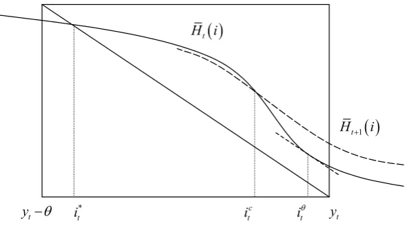
Consider an arbitrary datet where ¯Ht(i) gives rise to an interior equilibrium i∗t > yt−θ.
The objective in this section is to place an upper bound on the level of i∗
t that may be
In a generic period, it is possible for beliefs to fluctuate. Suppose the common belief is pessimistic and assigns a high probability to zt being low. A regime switch is
believed to be more likely at time t. This common belief would lead to a small delay in period t and a correspondingly large i∗
t, so that an absence of a regime switch would
imply a significant learning truncation in that period. Because it is common knowledge that fewer agents are investing and yet the regime still remains high, all agents become relatively more optimistic that the true fundamental is in fact favourable. If such a boost in optimism is sufficiently strong, it can in turn lead to a number of consecutive periods of maximum delay. In other words, pessimistic beliefs are reversed to optimistic ones by the absence of a regime change.
On the other hand, it is not inconceivable that ‘bubbles’ in the common belief may develop over time, leading agents to believe that a regime switch is just ‘around the corner’. That is, they are confident about a high regime today, whilst being convinced about a crash tomorrow. In a high regime, this would imply that the common knowledge density is highly skewed to the right. The skewness of the belief density, once obtained, may be persistent, leading to a similar pattern of play over time. In such a case, there would be large but occasional truncations, and the common knowledge evolution is characterised by spells of optimism (causing maximum delay) interrupted by occasional bursts of pessimism (leading to truncations). Because of this feedback effect, beliefs may cycle between optimistic and pessimistic phases.
The apparent instability of the common belief adds to the complexity of determin-ing ht explicitly over time. Nonetheless, some important quantitative implications for
hysteresis may be assessed without knowing the exact forms of ht. First, note that the
actual timing of a regime switch depends on the speed of yt evolution relative to that of
the common belief dynamics. Suppose that the agents’ beliefs fluctuate between a very brief but severe phase of pessimism and a long spell of optimism. If beliefs cycle at a very high speed relative to the dynamics of yt, then almost every visited state yt will be
tested against the severe pessimism phase. A regime switch therefore takes place as soon as the economy reaches the critical state yt that cannot be supported by the pessimistic
belief. Temporary delay therefore cannot lead to a significant hysteresis when beliefs evolve quickly.
Secondly, the assumption of a unique equilibrium at timet−1 clearly implies certain restrictions onht−1. These restrictions in turn place constraints on the form that ht may
take, and hence on the ensuing degree of delay at (arbitrary) datet. It turns out that the equilibrium uniqueness implies an upper bound on the degree of skewness of the belief density, and hence a lower bound on the degree of delay in any period, leading to the next key result.
t
y T
infZt * 1 t
i it*2 yt supZt
t
y i
T
1 t
H i
2 t
H i
kw l
%
l %
} l3%
kw3 } g}>
Kw3 l
]w3
} l
kw3 } g}=
kw kw3
kw3 w
kw3 kw3
]w3 lWw3 Kw3 l Kw3 l
Kw3 l Kw3 l
[image:23.595.153.441.86.248.2]w lWw3 |w3
Figure 3: A first-order stochastic dominant distribution leads to greater delay
t−1 and t. Then
i∗t ≤yt−θ+ε.
Proof. The objective is to derive an upper bound oni∗
t for any arbitrary datet, where no
restriction is imposed on ht and ht−1 except that they must yield a unique equilibrium
in period t and t−1. For i∗
t to take its maximum value, it clearly has to be an interior
solution, i.e. infZt< yt−θ. As learning truncations potentially take place prior to date
t, agents cannot believe zt to be too low and we must have infZt ≥ yt−θ−ε, thus in
sum infZt ∈ [yt−θ−ε, yt−θ). On the other hand, because equation 5.6 always holds
(as a consequence of claim1; see the discussion following section5.1) and εis big relative to one, it follows that supZt> yt for any timet after a regime switch. Let us consider an
arbitrary fixed pair of infZt and supZt that satisfy such constraints. Suppose that two
distributions over the fixed support Zt are rankable in the sense of first-order stochastic
dominance. Under the assumption that there is a unique equilibrium in period t, it follows from a simple graph-theoretic argument (see figure3) that the distribution which first-order stochastically dominates the other leads to a smaller equilibrium i∗
t. Thus, i∗t
is at its greatest if the underlying distribution ht is first-order stochastically dominated
by all other possible distributions within the class of interests. If any distribution ht is
possible, then the upper bound for i∗
t is uninterestingly given by yt with the underlying
distribution being ¯Ht−1(i) = 0,∀i. The next step of our proof is to characterise the class
of distributions of interests, namely those which are consistent with a unique equilibrium at each date t−1 and t.
For convenience, we reproduce equation3.9
ht(i) =
1 2ε
Z i+ε
z=i−ε
˜
and define
e
Ht−1(i)≡
Z supZt−1
z=i
˜
ht−1(z)dz. (4.8)
Ashtis related to ˜ht−1according to equation3.9, the first step is to characterise the class
of ˜ht−1 consistent with a unique equilibrium in period t−1. Recall from equation 3.7
that ˜ht−1 is either identical toht−1 or is a left-sidedly truncated version of it, depending
on whether infZt−1 ≥i∗t−1. In terms of the c.d.f, this corresponds to Het−1(i)≥H¯t−1(i).
Consider two possibilities in turn. First, if Het−1(i) = ¯Ht−1(i) then there is no truncation
in periodt−1, implying that the equilibrium is a corner solution ofi∗
t−1 =yt−1−θ. Because
there is no other equilibrium, Het−1(i) and ¯Ht−1(i) must lie above (yt−1−i)/θ for all
i ∈ (yt−1−θ, yt−1]. On the other hand, if Het−1(i) >H¯t−1(i) then there is a truncation
in period t − 1 and Het−1(i) > H¯t−1(i) > (yt−1 −i)/θ for i > i∗t−1 and Het−1(i) =
1 > (yt−1−i)/θ for i ∈ yt−1−θ, i∗t−1
. Hence conditional on there being a unique equilibrium in period t−1, one can conclude that Het−1(i) must lie above (yt−1−i)/θ
everywhere except perhaps at the singular point i = yt−1 −θ. Let us call the class of
distributions Het−1(i) with such property the uniqueness class.
For any fixed supportZt, there corresponds a uniqueZet−1 ≡[infZt+ε,supZt−ε].
On the supportZet−1, let us define, for a small e >0, a benchmark distribution
˜
het−1(i)≡
1
θ, for i∈[yt−1 −θ+e, yt−1+e] ,
and zero otherwise, with the corresponding c.d.f.
e
Hte−1(i)≡
yt−1 −i
θ + e θ.
Clearly lime→0Hete−1(i) is first-order stochastically dominated by all other distributions in
the uniqueness class. Recall from the proof of3that the shock transition rule in equation
3.9 preserves the first-order stochastic dominance ordering. In other words, ase→0, the benchmark density ˜he
t−1 generates a belief density at timet, sayhet, that is stochastically
dominated by all other densities ht which are a shock transition rule of the uniqueness
class. Hence, an upper bound on i∗
t is simply the limit as e→0 of the solution to
¯
Hte(i)≡
Z supZt
z=i
het(z)dz =
yt−i
e
1
inf t
t Z
y T e
H H t
y i T
e
t H i
1
e t H i
e t h i e t h i
1
[image:25.595.137.441.91.478.2]T
Figure 4: Construction of ¯He
t and het
where
het(i) =
1 2ε
Z i+ε
z=i−ε
˜
het−1(z)dz
=
1
θ for i∈[yt−θ+e+ε, yt+e−ε]
i−(yt−θ+e−ε)
2εθ fori∈[yt−θ+e−ε, yt−θ+e+ε]
−i+(yt+e+ε)
2εθ for i∈[yt+e−ε, yt+e+ε]
.
Figure4 illustrates the construction of ¯He
t and het.
It can be readily checked that ¯He
t (i) = Hete−1(i) for i ∈ [yt−θ+e+ε, yt+e−ε]
and ¯He
t (i) > Hete−1(i) for i > yt+e−ε, hence the fixed point solution to equation 4.9
must lie in the interval [yt−θ, yt−θ+e+ε]. Take the limit e→0, and the proposition
is proved.
Sinceεis small relative toθ, proposition2states that there is a significant hysteresis in equilibrium. Significant hysteresis in both regimes in turn suggests that the state variable yt can cycle, even if there is no actual change in the fundamental variable zt. A
high regime persists and yt tends to rise, until yt =zt∗+θ is reached, inducing a regime
back to high. Even if there is in fact no change in zt, yt tends to fluctuate in a unique
equilibrium cycle.
Proposition 2 sheds light on the equilibrium properties, allowing us to verify con-jectures 1,2 and 3 made earlier.
Claim 8. Conjectures 1, 2 and 3 are satisfied in equilibrium.
Proof. Suppose that there is a regime switch from low to high in period −1, so that Z−1 =
i∗
−1,supZ−1
. Because of the model’s symmetry with respect to the regimes, proposition 2 adjusted for a low regime implies that i∗
−1 ≥y−1−ε. Because of learning
truncations, we also have supZ−1 ≤y−1+ε. Thus
Z0 =
i∗−1−ε,supZ−1+ε
⊆ [y−1−2ε, y−1+ 2ε]
so that
|Z0| ≤4ε≪θ
validating conjecture 1. Next, note that
σ2 0
ε2 = Z
z∈Z0
z−µ0
ε
2
h0(z)dz.
Since µ0 ∈Z0, it follows that for any z∈Z0
z−µ0
ε ≤
|Z0|
ε ≤4.
Thus σ2
0/ε2 < ∞ and conjecture 2 is verified. Lastly, i∗−1 ≥ y−1 −ε > y−1 −θ +ε and
hence conjecture 3 is satisfied.
5
Equilibrium Uniqueness Conditions
We now detail the conditions under which equilibrium uniqueness can be guaranteed, and verify whether these conditions are met.
5.1
Contraction arguments
A sufficient condition for uniqueness can be based on contraction mapping condition:
− ∂
∂iH¯t(i)< 1
When this condition holds, it is clear that there is a unique solution to equation 3.5. Using Leibniz’s rule on equation 3.6 gives
− ∂
∂iH¯t(i) =ht(i), (5.2)
so that the uniqueness condition5.1 is simply
max
i∈[yt−θ,yt]
ht(i)<
1
θ. (5.3)
In general, uniqueness requires the beliefs aboutz∗
t to be sufficiently diffuse, and condition 5.3 gives one measure of such diffusion in terms of the sup-norm of the belief posterior.
While the sufficient condition based on sup-norm contraction can be a powerful tool, it will prove to be too strong in the present case. Intuitively, beliefs aboutz∗
t in the first
few periods immediately after a regime switch will be relatively precise, and condition5.3
may only hold whenεis restricted to be very large relative toθ. Whenεis small relative to θ, which is the main case of interest, it will be shown in section 5.3 that even after a large number of belief updates, the condition still cannot be guaranteed although the equilibrium may well be unique. A less demanding condition for uniqueness is therefore required.
Consider an alternative criterion, related to the degree of concavity of ¯Ht(i). Note
that by an argument that is topologically equivalent to a contraction mapping, if ¯Ht(yt)>
0, then the concavity everywhere of ¯Ht(i) ensures a unique equilibrium. Similarly, if
¯
Ht(yt−θ) < 1, then an everywhere convex ¯Ht(i) implies uniqueness. In general, of
course, ¯Ht(i) is only concave on a certain set and convex otherwise. But suppose that
one starts in a high regime and that ¯Ht(yt) > 0, then it is easy to see that a unique
equilibrium ensues if
whenever ¯Ht(i) is convex, ¯Ht(i)>
yt−i
θ . (5.4)
The condition can also be equivalently expressed as follows. Restrict attention to the range of i for which ¯Ht(i) is convex, and define iθt by the solution8 to
− ∂H¯t(i)
∂i
iθ
t
=ht iθt
= 1 θ
then there is a unique equilibrium if
¯ Ht iθt
> yt−i
θ t
θ . (5.5)
8Since
htis always unimodal, there is a unique such solution if one restricts attention to the convex
t
iT yt
t
H i
t
y T * t
i
1
t
H i
c t
i
Kw Kw
Kw lw A
|wlw
=
l
w kw lw @
kw l ? @ l
Kw |w A w
[image:28.595.152.446.86.250.2]Kw
Figure 5: A convexity-based condition for a unique equilibrium, and the first right crossing between ¯Ht+1 and ¯Ht.
Figure 5 depicts how the ‘bounded convexity condition’ condition 5.5 implies a unique equilibrium. The condition supplements the bounded sup-norm in equation5.3. Clearly, if there is no solution iθ
t to ht iθt
= 1/θ, then it must follow that ht(i)< 1/θ for all i,
and the bounded sup-norm condition 5.3 is satisfied.
The prerequisite that ¯Ht(yt)>0 for all t (if one is in a high regime) is intuitively
a requirement that agents must always believe that the decisive agent has a dominant strategy with a positive probability. In fact, for ¯Ht(yt) to be larger than 0 for all t in a
high regime, it is sufficient to show that ¯Ht(yt) > 0 at the starting date of the regime
(i.e. in the period after the regime switches from low to high). This is becauseε is large relative to 1 and agents continue assigning positive weights to fundamental exceeding yt
as long as the high regime continues. Intuitively, it is immediately after a regime switch and a transition that follows, that the information about the fundamentals is closest to being complete. The applicability of global game technique relies on the shock transition rule to introduce enough uncertainty in this stage. If after a transition, all agents believe with probability one that the true fundamental variable lies within a set defining some coordination game, then the iterated dominance argument fails and there is a multiplicity. The common belief support must therefore be large enough so that the fundamental lies in the dominance region with some probability.
Claim 1 can be used at this point to show that this condition is always satisfied. More concretely, let us suppose that there is a regime switch from high to low at date t.9 The objective is to prove that ¯H
t+1(yt+1−θ) >0, as we now explain briefly. In the
beginning of period t+ 1 agents believe that z∗
t+1 is distributed over [infZt−ε, i∗t +ε],
where bothi∗
t andZt are common knowledge. If infZt−ε > yt+1−θ, then agents believe
9We change our convention and choose a low regime as the starting point here so that claim1 may
with probability one that z∗
t+1 ∈[yt+1−θ, yt+1], so that the decisive group of agents will
definitely play a coordination game in periodt+ 1 and there must be a multiplicity. Thus a necessary condition for uniqueness in the first period given that the regime just switches to low is that
infZt−ε < yt+1−θ (5.6)
which is identical to ¯Ht+1(yt+1−θ)>0. That this condition is always satisfied can now
be verified using claim 1. Consider date t at which there is a regime switch from high to low. The equilibrium at that date is either a corner solution (i∗
t = yt−θ) or interior
(i∗
t > yt −θ). If it is a corner solution, then the fact that zt∗ ≥ infZt ≥ yt−θ must
imply that z∗
t = yt − θ for there to be a regime switch. Thus the true z∗t becomes
common knowledge, i.e. Zt = {zt∗}.10 It follows that, in period t + 1, agents believe
that z∗
t+1 ∈[z∗t −ε, zt∗+ε] = [yt−θ−ε, yt−θ+ε]≈[yt+1−θ−ε, yt+1−θ+ε], so that
z∗
t −ε ≈ yt+1 −θ−ε < yt+1−θ and the condition 5.6 is satisfied. On the other hand,
suppose more generally that the equilibrium is interior. Then it follows from the claim that infZt< yt−θ, and hence infZt−ε < yt−θ−ε≈yt+1−θ−ε < yt+1−θ, and again
the condition is satisfied.
5.2
A recursive condition
The procedure for checking equilibrium uniqueness can be summarised as follows. If the bounded sup-norm condition in equation 5.3 is satisfied, then there is a unique equilibrium, otherwise we proceed to check if both ¯Ht(yt)>0 and the bounded convexity
condition in equation 5.5 hold. When all conditions fail, it is concluded that there is a multiplicity. Analogous conditions can be written down for the case where the initial regime is low.
Given the dynamic nature of the common belief, it must be determined how the equilibrium uniqueness considerations develop over time. Towards this end, it would be useful to have a set of sufficient conditions under which uniqueness can be implied recursively, namely that uniqueness in period t would imply uniqueness in period t+ 1. Let us refer to such a set of sufficient conditions as the recursive condition for short. For example, the first-order stochastic dominance is a recursive condition; ¯Ht+1 being greater
than ¯Ht everywhere is sufficient to ensure that condition 5.4 is recursive, provided that
¯
Ht+1−H¯t is large relative to 1/θ (which holds since θ is assumed large). However, this
particular recursive condition is of limited use, as it obviously cannot be met for all t, e.g. under a pure transition, ¯Ht+1 must cross ¯Ht at least once for any ¯Ht. Intuitively,
equilibrium uniqueness is recursive in this case because the first-order stochastic domi-nance rules out additional equilibria where agents attack the existing regime earlier, by
10This is precisely the singular case mentioned earlier in which the information about the fundamentals
requiring the common belief to become more biased in favour of greater delay.
The essential property of a recursive condition is that the common belief in each period must become sufficiently more diffuse over time, so that there does not exist addi-tional equilibria on which agents can coordinate. Specifically, in view of the uniqueness condition5.5, the shock transition rule must lead to a ‘convexity contraction’11, so that the validity of iterated dominance can be inferred recursively; namely ¯Ht iθt
> yt−iθt
/θ implies ¯Ht+1 iθt+1
> yt+1−iθt+1
/θ.
Let us construct a recursive condition with such property. Suppose that at time t, the regime is high and the bounded convexity condition 5.5 is met. Consider figure
5 again, where both ¯Ht and ¯Ht+1 are plotted. As we have not ascertained if ¯Ht may
cross ¯Ht+1 several times in general, let ict denote the point at which ¯Ht+1 crosses ¯Htfrom
the right for the first time (and necessarily from above), so that ¯Ht+1(i)>H¯t(i) for all
i > ic
t.12 Note that uniqueness in period t implies that ¯Ht(i)>(yt−i)/θ for all i > i∗t.
The strategy is to exploit this fact and work out the conditions under which ¯Htcan serve
as a lower bound for ¯Ht+1 atiθt+1, i.e. the point where−∂H¯t+1/∂i= 1/θ. In other words,
we seek to establish conditions under which we are able to write
¯
Ht+1 iθt+1
> H¯t iθt+1
(5.7)
> yt−i
θ
t+1
θ (5.8)
≃ yt+1−i
θ
t+1
θ
and hence conclude that there is a unique equilibrium in period t+ 1.
A construction of a recursive condition amounts to obtaining two sufficient condi-tions that ensure inequalities 5.7 and 5.8 are both satisfied. Since ¯Ht+1(i) > H¯t(i) for
all i > ic
t, a sufficient condition for inequality 5.7 to hold is that iθt+1 > ict. On the other
hand because there is a unique equilibrium in period t, for inequality 5.8 to hold, it is sufficient and necessary that iθ
t+1 > i∗t. Thus, a recursive condition is simply given by
iθt+1 >max{i c
t, i∗t}. (5.9)
There exists a variety of sufficient conditions that would guarantee that this recur-sive condition holds. For instance, a condition may be rewritten in terms of the density.
11
Namely the bounded convexity condition must be recursive, so that when condition5.5 is met in periodt, it is also met in periodt+ 1. On the other hand, a shock transition rule always implies a sup-norm contraction in the belief density. To see this, recall that a shock transition rule ofht(z) is merely
its average over the interval [z−ε, z+ε]. Clearly, on any fixed interval, the average cannot exceed the supremum. Hence, the supremum of averages ofhtcannot exceed the supremum ofhtitself.
12This is a slight abuse of notation, as ic
t was defined earlier in lemma 2 as any crossing point. No
Because of the unimodality ofht+1, a sufficient condition for iθt+1 >max{ict, i∗t} is that
ht+1(max{ict, i∗t})>
1
θ. (5.10)
Alternatively, a condition based on the mode im
t may be constructed. Suppose that we
always haveic
t > i∗t, so that one only needs to showiθt+1 > itc. Sinceiθt+1 > imt+1, a sufficient
condition for iθ
t+1 > ict comprises two inequalities
im
t+1 ≥imt > i c
t. (5.11)
5.3
Verifying uniqueness
Somewhat surprisingly, an implication of the limiting result in equation 4.1 is that the equilibrium uniqueness prior to the first truncation cannot be guaranteed by the sup-norm contraction condition 5.3 alone no matter how large is the number of pure shock transitions. As ht(z∗) is unimodal and attains its maximum at z∗ = E(zt∗) = µ0, we
have
supht≈
2π σ02+tε2/3
−1
2 . (5.12)
Thus, a sufficient condition for uniqueness according to equation 5.3 is given by
θ <
q
2π(σ2
0 +tε2/3) (5.13)
t > 3 (θ
2−2πσ2
0)
2πε2 .
The right hand side of equation5.13 is the minimum number of pure transitions required before uniqueness can be guaranteed by the sup-norm contraction condition in equation
5.3. By claim7, the expected number of periods before the first truncation is proportional to θ/ε, whilst the right hand side of equation 5.13 is of the order (θ/ε)2. In other words, the first truncation takes place before the contraction condition can be satisfied. Therefore, in ensuring uniqueness in the case of pure transitions, the convexity contraction condition must be used.
It is instructive to consider two distinct phases of the learning process separately, and derive uniqueness conditions for each case. The first phase of learning starts in the period immediately after a regime switch. In this phase, subject to the initial belief, agents update their common belief using the shock transition rule alone. After sufficiently many periods of pure shock transition rules, the common belief approximately follows a normal distribution by the central limit theorem. This marks the start of the second phase, which continues until the first learning truncation and subsequently the regime switch. Each phase is now considered in turn.