Effect of Quality Parameters in Efficient Routing Protocol – Grid FSR with Best QoS Constraints

Effect of Quality Parameters in Efficient Routing

Protocol – Grid FSR with Best QoS Constraints

S. Nithya Rekha

Scholar

Dept. of Computer Science Periyar University

Dr. C. Chandrasekar

Periyar University

R. Kaniezhil

Scholar

Dept. of Computer Science Periyar University

ABSTRACT

Rapid advanced in information technology has made it possible to transmit the data in wireless links without the aid of any fixed infrastructure or centralized administrator. Wireless mobile ad hoc networks are creating, administering and organizing entities. Thus a set of self-motivated mobile wireless users is able to dynamically exchange data among themselves, even in the absence of a predetermined infrastructure and controller. In our research work, we present investigations on the behavior of the Proactive Routing Protocol FSR in the GRID by analysis of various parameters. The Performance metrics that are used to evaluate performance of the routing protocols are Packet Delivery Ratio (PDR), Network Control Overhead, Normalized Overhead, Throughput and Average End to End Delay. Experimental results reveal that FSR is more efficient in Grid FSR in all QOS constraints.FSR can be used in all Resource critical environments. Scalability in respect to QOS is effective in FSR- large area routing protocol. Grid Fisheye state routing (GFSR) consumes less bandwidth by restricting the propagation of routing control messages in paths formed by alternating gateways and neighbor heads, and allowing the gateways to selectively include routing table entries in their control messages.PDR and Throughput are 100% efficient in Simulation Evaluation with NS2.

General Terms

MANET, Grid FSR Protocol, NS2, Simulation Results.

Keywords

MANET, Network Protocols, Link State Routing (LSR), Fish-eye State Routing Protocol (FSR), GRID Fisheye Routing Protocol (GFSR), QoS, NS2, Packet Delivery Ratio, Throughput, Control Overhead, Normalized Overhead, End to End Delay.

1.

INTRODUCTION

In areas in which there is little or no communication infrastructure or the existing infrastructure is expensive or inconvenient to use, wireless mobile users may still be able to communicate through the formation of an ad hoc network [1] [2]. J. Broch, D.A. Maltz, D.B. Johnson, Y.-C. Hu, and J. Jetcheva, 1998 et al. , proposed that Mobile ad hoc networks (MANET) consists of a collection of wireless mobile nodes, which dynamically exchange data among themselves without the reliance on a fixed base station or a wired backbone network, it have potential use in a wide variety of disparate situations such as responses to hurricane, tsunami, earthquake, emergency relief, terrorism and military operation.

In [1], the author proposed that Mobile Ad-hoc Network (MANET) is a self configuring network composed of mobile nodes without any fixed infrastructure. In a MANETs, there are no difference between a host node and a router so that all nodes can be source as well as forwarders of traffic. Moreover, all MANET components can be mobile. They provide robust communication in a variety of hostile environment, such as communication for the military or in disaster recovery situation when all infrastructures are down. A very important and necessary issue for mobile ad hoc networks is to finding the root between source and destination that is a major technical challenge due to the dynamic topology of the network. Routing protocols for MANETs could differ depending on the application and network architecture.

1.1 Brief Review of Routing Protocols

The primary goal of routing protocols in ad-hoc network is to establish optimal path (min hops) between source and destination with minimum overhead and minimum bandwidth consumption so that packets are delivered in a timely manner. A MANET protocol [1] should function effectively over a wide range of networking context from small ad-hoc group to larger mobile Multi hop networks.

1.2 Proactive Routing Protocols

In proactive routing protocols each node keeps the routing information in a number of tables. This information is exchanged with other nodes periodically and/or when there is a change occurs in the network topology. A number of proactive routing protocols have been proposed. Some of these protocols are DSDV, WRP, GSR, HSR, FSR, OLSR, CGSR, STAR, MMWN etc. among which FSR and OLSR scale very well in large and highly mobile network. All these protocols differ in the way they update routing information, the number of tables and the type of information in the tables.

The rest of this paper is organized as follows: First of all, we make a brief survey on FSR and Protocol Operation in section II. In section III, a survey on GRID in FSR, In Section IV , description on how GFSR works. Section V presents the performance evaluation and section VI concludes the paper.

2. RELATED WORK

2.1 FSR (Fisheye State Routing)

neighbors with a frequency which depends on distance to destination. From link state entries, nodes construct the topology map of the entire network and compute optimal routes. Simulation experiments show that FSR is simple, efficient and scalable routing solution in a mobile, ad hoc environment. Figure 1 refers the fisheye scope with different hops.

Fig 1: Fisheye Scope

In [18], the authors proposed that, Fisheye State Routing (FSR) protocol is a proactive (table driven) ad hoc routing protocol and its mechanisms are based on the Link State Routing protocol used in wired networks. FSR is an implicit hierarchical routing protocol. It reduces the routing update overhead in large networks by using a fisheye technique [3]. Fish eye has the ability to see objects the better when they are nearer to its focal point that means each node maintains accurate information about near nodes and not so accurate about far-away nodes. The scope of fisheye is defined as the set of nodes that can be reached within a given number of hops. The number of levels and the radius of each scope will depend on the size of the network. Entries corresponding to nodes within the smaller scope are propagated to the neighbors with the highest frequency and the exchanges in smaller scopes are more frequent than in larger. That makes the topology information about near nodes more precise than the information about farther nodes. FSR minimized the consumed bandwidth as the link state update packets that are exchanged only among neighboring nodes and it manages to reduce the message size of the topology information due to removal of topology information concerned far-away nodes. Even if a node doesn’t have accurate information about far away nodes, the packets will be routed correctly because the route information becomes more and more accurate as the packet gets closer to the destination. This means that FSR scales well to large mobile ad hoc networks as the overhead is controlled and supports high rates of mobility. The FSR concept originates from Global State Routing (GSR) [19]. GSR can be viewed as a special case of FSR, in which there is only one fisheye scope level and the radius is infinite. As a result, the entire topology table is exchanged among neighbors. Clearly, this consumes a considerable amount of bandwidth when network size becomes large.

2.2 Advantages of FSR Protocol

The followings are the advantages of FSR Protocol over most of the other MANET routing protocols [3],

 Simplicity

 Usage of most up to date shortest routes  Robustness to host mobility

 Exchanges partial routing updates with the neighbors

 Reduced routing update traffic

2.3 FSR Routing Protocol has the following

characteristics

 Each node maintains another node’s list of broadcast updating information, which is using useful for network topology in FSR updating and can also avoid routing loop.

 Different fisheye fields use different broadcast links with different frequencies to update information, thus reducing the routing overhead.

 The router in every communication is that according to the information of topology, the shortest path of algorithm is calculated, and nearer to the destination, the more accurate will be the routers information.

 When the link breakdowns, the protocol will directly delete the relevant information in the neighbor list and the topology list without broadcasting any controlling information.

2.4 Protocol Operation

Fisheye State Routing is a table-driven or proactive routing protocol. As mentioned, FSR is based on link state routing and it is able of immediately providing route information when needed. FSR is functionally similar to LS as it maintains a full topology map at each node. The link state packets are exchanged periodically instead of event driven. The topology tables are sending to local neighbors only (instead of flooding the entire network) Sequence numbers are used for entry replacements as well as for providing loop-free routing. The fisheye scope message updating scheme is highly accurate for inner scope nodes as entries in the routing table corresponding to nodes within the smallest scope are send to the neighbors with the highest frequency. For outer scope nodes, information may blur due to longer exchange interval but there is no need to "find" the destination firstly (as in on-demand routing).The fisheye scope technique allows exchanging link state messages at different intervals for nodes within different fisheye scope distance, leading to a reduction of the link state message size.

2.4.1 Topology Table

The Topology table is created by using the topology information obtained from the link state messages. Each destination has an entry in the table (full topology map). An entry consists of two parts: the link state information and a destination sequence number. Based on this table, the routing table will be calculated. The distance information will then be obtained from the routing table calculation. It is used to classify the node to a fisheye scope. The topology table has following entries for every link state entry: - Destination Address

- Destination Sequence Number - Link State List

2.4.2 Neighbor Link State List

On receiving a link state message, a node records/updates the sender in its neighbor list.

If nothing is received for a timeout interval, the corresponding station will be removed from the neighbor list.

The following information is maintained for each neighbor node:

2.4.3. Routing Table

The routing table provides next hop information to forward a packet to a destination in the network. The entries are updated on a topology table change. The routing table consists of the following fields:

- Destination Address - Next hop address -Distance

The inaccuracy for far away nodes will increase in a mobile environment but a packet approaching its destination finds more and more accurate routing instructions as it enters sectors with higher refresh rates.

3. GRID based Fisheye State Routing

Protocol (GFSR)

Fisheye state routing protocol improves traditional link-state routing in the MANET. By adopting the idea of GRID [4] in FSR, we proposed an efficient GRID-based fisheye state routing protocol (GFSR). GFSR provides the advantage of less control message exchange and more bandwidth to transmit data. A hierarchical architecture is used in GFSR. A gateway is elected in each grid and is the only node in the grid to exchange control messages and data packets with other grids. Substantial bandwidth can be saved in this way. Simulation shows that GFSR is more efficient than FSR, especially in high-density networks. Although fisheye state routing could reduce control message overhead, the bandwidth usage is still inefficient when the node density is high. By integrating the mechanism of GRID into FSR, only fewer mobile nodes called gateways should be responsible for exchanging update messages and routing. It can reduce message overhead further. We can propose a virtual grid-based routing protocol called GFSR to make communication more efficiently under highly-density environment.

3.1 Basic idea

T-H. Chu and S-I. Hwang, et al., 2006, proposed that GRID-Based Fisheye State Routing (GFSR) Protocol is an extension to Fisheye State Routing. By adopting the idea of GRID into Fisheye State Routing, fewer forwarding nodes can lower the cost of control messages and can save bandwidth for data transmission. This makes transmission more efficiently, especially in high-density networks. In high-density networks, many collisions may occur. When there are more nodes existent in the radio transmission range, more interference will occur. If the number of forwarding nodes in a certain square can be reduced, less interference and collisions occur and more bandwidth can be saved.

3.2 GRID architecture

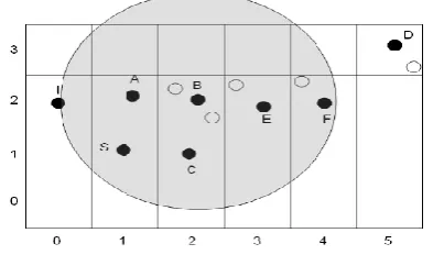
We assume that each node in ad hoc networks has installed a GPS receiver. Through GPS devices, nodes can easily derive their location information. The geographic area of an ad hoc network is partitioned into two dimensional virtual grids and each grid has its unique coordinate number (x, y). As illustrated in Figure 2, each node can calculate in which grid it currently dwells based on the physical location information derived from GPS. In [4] ,initially, a gateway election is held in each grid, where a gateway is the node responsible for maintaining the routing table in its grid, and for exchanging routing information using fisheye state routing scheme. The node nearest to the physical center of a grid is a good candidate as a gateway. The grid length in GRID architecture

can be set in a such way that the transmission range of each gateway can effectively cover its eight neighbor grids. Therefore, any mobile node knows the gateways of its eight neighbor grids. As illustrated in Figure 3, the black-dottted nodes denote gateways and the large gray circle represents the transmission range of node B.

Y axis

X-axis

Fig 2: The square is divided into many logical grid

Fig 3: Transmission range of each gateway could cover eight neighbor grids

4. PROPOSED WORK

4.1 Routing Scheme

Each gateway maintains a Routing table by the routing information which is exchanged periodically. When a node needs to transmit data, it checks whether it is a gateway or not. If it is a gateway, it transmits data to next hop by checking its routing table. If it is non-gateway node, it just sends data to its gateway, and then the gateway will take over to forward the message to next hop.

In Figure 4, the gateways along the routing path will check the destination and determine who the next hop should be. When a packet approaches nearer to its destination, the routing information stored in the gateways becomes progressively more accurate. Packets finally arrive at the grid of destination node. If destination is a gateway, the packet is received by that gateway. Otherwise, the gateway forwards the packet to the destination node in its grid.

Initially before data transmission each grid broadcast its grid member’s information through gateway node. So that each gateway can exchange its grid members list. So whole network comes under the communication. While data transmission between grid members to other node gateway maintains unicast transmission until reaches its destination.

…

…

(0,0)

(0,0)

…

(0,1)

(1,0)

(0,0)

…

Through this method we propose that there will be no packet loss from source to destination.

4.2 Grid Formation Calculation

Distance between Nodes (DBN) is calculated with the following Equation.

sl_x = MAX-X / X-SCALE + 1 sl_y = MAX_Y / Y-SCALE + 1

X-Grid = i< sl-x x < = I * scale && x > = (I – 1) * x scale

Y-Grid = i<=sl-y y < = I * y –scale && y >= (I – 1) * y scale

grid – id = (x_grid – 1) x (sl – x + y_grid )

DBN =



 







n

i n

i

j i j

i

x

y

y

x

1 1

2 2

)

(

)

(



i

,

j

Design and implementation of communication protocols and algorithms, the use of simulation tools provides a substantial productivity and allows near perfect experimental control in various wireless networks.

Fig 4 : GRID Architecture with Unicast data path from Source node to Destination Node

Grid Gateway

Source Node

Destination Node

Grid

--- Unicast Data Path

5. SIMULATION RESULTS

To evaluate the performance of routing protocols, both qualitative and quantitative metrics are needed. Most of the routing protocols ensure the qualitative metrics. Therefore, we can use four different quantitative metrics to compare the performance. The proposed GFSR protocol is implemented using NS2 simulator. The performance is measured according to (1) Packet Delivery Ratio with nodes (2) Control message overhead with nodes (3) Normalized Overhead with nodes (4) End to End Delay with Nodes.

Measurement Parameters

The performances o f r o ut ing p ro to col s (F SR and GF S R ) ar e compared using the following important Quality of Services (QoS) metrics:

5.1 Packet Delivery Ratio (PDR) Versus

Nodes

Packet delivery ratio is an important metric as it describes the loss rate that will be seen by the transport protocols, which run on top of the network layer. Thus packet delivery ratio in turn reflects the maximum throughput that the network can support. It is defined in as the ratio between the number of packets originated by the application layer CBR sources and the number of packets received by the CBR sink at the final destination.







send N

recv

CBR

CBR

PDR

1 1

where N is the number of data sources, CBR recv is the total number of CBR packets received and CBR send is the total number of CBR packets sent per source.The fraction of packets sent by the application that are received by the receivers. The number of data packets sent from the source to the number of received at the destination. As the calculation, PDR = (control packets sent-delivery packet sent)/control packets sent. The result of Packet delivery ratio is illustrated in Figure 5 with 100% efficiency without any packet loss. In FSR, all nodes exchange information in different density environment. When density grows bandwidth is used to exchange more and more routing packets. At the same time GFSR has the fixed number of gateways in the square. Hence control messages are restricted to a limited extend. so the bandwidth can be saved to transmit data packet.

Fig 5: Packet Delivery Ratio V/s Number of Nodes (FSR & GFSR)

becomes highly crowded. Hence PDR is 100% efficient in GFSR with 150 nodes than FSR.

5.2 Control Message Overhead Versus

Nodes

Network Control overhead (NCO) [12] [21], is used to show the efficiency of the MANET’s routing protocol scheme. It is defined, as the ratio of the number of control messages (the number of routing packets, Address Resolution Protocol (ARP), and control packets e.g., RTS, CTS and ACK) propagated by each node throughout the network and the number of the data packets received by the destinations. The definition is:

NCO = Number of Control Message Sent

Number of data Received

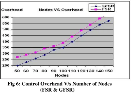
From Figure 6, it is observed that the network control overhead needed for FSR routing protocol goes down as the data rate increases. This occurs because nodes wait a longer time before transmitting Link State Packets (LSPs) it received from other nodes at each successive scope. This results in lower control overhead traffic. The reductions of network control overhead at higher data rate are very significant. This is because the same amounts of routing and control message are needed to route CBR traffic at lower data rate as well as at higher data rate. In GFSR, the control overhead can be reduced substantially. If there are n grids, there are n grids, there are at most n nodes need to exchange routing information. The control messages are exchanged periodically. The result of control overhead is shown in Fig. Therefore, in Figure 6, control message overhead only grows slowly. Note that the message overhead still increases with the number of nodes. The reason is that there are messages used to maintain the grid architecture. More nodes need more maintenance messages.

Fig 6: Control Overhead V/s Number of Nodes (FSR & GFSR)

5.3 Normalized Overhead versus Nodes

The graphs in Figure 7, illustrate the Normalized routing overhead experienced in the 1000 m X 1000 m boundary. As Figure clearly explains that in GFSR normalized overhead is comparatively reduced than FSR. In our simulation, the maximum update interval for the intrascope and interscope is set to be half of that of FSR. The routes produced would have been less accurate which may have result in a drop in throughput.

This means that accuracy of the routes will be high during high mobility where nodes are more likely to migrate more frequently and experience topology changes, and when

mobility is low, less updates are sent. From the result shown in Figure 7, it can be seen that GFSR produced less overhead than FSR, across all different level of node density.

Fig 7: Normalized Overhead V/s Number of Nodes (FSR & GFSR)

5.4 Average End-to-End Delay Versus

Nodes

End-to-end delay indicates how long it took for a packet to travel from the source to the application layer of the destination. Here again GFSR has low delay comparied to FSR.The result in figure 8, shows that GFSR’s each data packet experiences lower end-to-end delay than in FSR. The lower delay experienced is due to the higher level of accessibility to the wireless medium. This is because in our proposed strategies each node generates less route updates than in FSR, which means there is less contention for the channel when a data packet is received. Therefore, each node can forward the data packet more frequently.

5.5 Throughput Versus Nodes

Fig 9: Throughput V/s Number of Nodes (FSR &GFSR)

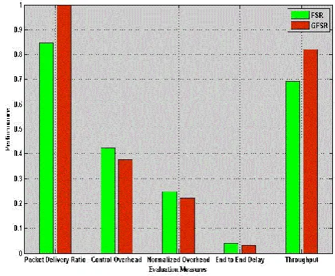
Fig 10: Average Comparison of FSR and GFSR in Performance Metrics using Simulation

Table 1: Comparative Analysis of FSR and GFSR in NS2

Nodes

Packet Delivery Ratio

Control Overhead

Normalized Overhead End to End Delay Throughput

FSR GFSR FSR GFSR FSR GFSR FSR GFSR FSR GFSR

50 88.0 100.0 275 200 0.16167 0.11758 0.03154 0.02654 72.132 81.968

75 87.0 100.0 315 275 0.18519 0.16167 0.03756 0.02856 71.312 81.968

100 85.0 100.0 385 350 0.22634 0.20576 0.04248 0.02878 69.672 81.968

125 83.0 100.0 515 475 0.30276 0.27925 0.04595 0.03434 67.213 81.968

150 80.0 99.882 628 578 0.36921 0.34020 0.04917 0.03769 65.574 81.871

6. CONCLUSIONS

Table 1 explains the Comparative Analysis of FSR and GFSR in NS2. This research studies compares FSR and GFSR routing protocols for MANETs. FSR is also an implicit hierarchical routing protocol. Packet delivery ratio and Network control overhead are very important when deciding how reliable a protocol is and how good it performs. Network control Overhead is a measure of how effective a protocol is. A routing protocol must be both reliable and efficient when it is used in energy- constrained wireless networks with very limited bandwidth. In our Simulation Evaluation terms of Packet delivery ratio and Throughput in GFSR Out performs FSR with 100% without packet loss with lower delay. In this paper, we proposed a new routing scheme called Grid FSR. At the cost of a little longer routing path, GFSR provides a highly efficient solution with lower control message overhead and fewer routing nodes which are responsible for exchanging routing information. In high-density environments, our

method exhibits low interference and fewer collisions and it leads to more efficient communication among mobile nodes.

In future, various mobility models can be used to compare various parameters with respect to increase in number of nodes used. The performance differentials in this simulation are investigated using varying Packet Delivery Ratio, Control Overhead, Normalized Overhead, Throughput and End to End Delay with respect to Number of Nodes. On the other hand, number of nodes is increased from 100 nodes to 150 nodes. Based on the simulation results, how the performance of protocol can be improved is also recommended. Comparative analysis of simulation results includes network performance with mobile node speeds and network size. Simulations of protocols to analyze their performance in different conditions were performed in NS2 simulator. Finally GFSR outperforms and shows its average efficiency in all Simulation parameters in below figure 10.

7. ACKNOWLEDGEMENT

8. REFERENCE

[1] J. Broch, D.A. Maltz, D.B. Johnson, Y.-C. Hu, and J. Jetcheva, “A Performance Comparison of Multi-Hop Wireless Ad Hoc Network Routing Protocols,” In Proceedings of ACM/IEEE MOBICOM’98, Dallas, TX, Oct. 1998, pp. 85-97.

[2] T.-W. Chen and M. Gerla, “Global State Routing: A New Routing Scheme for Ad-hoc Wireless Networks,” In Proceedings of IEEE ICC’98, Atlanta, GA, Jun.1998, pp. 171-175.

[3] G. P. Mario, M. Gerla and T-W Chen, “Fisheye State Routing: A Routing Scheme for Ad Hoc Wireless Networks, “Proceedings of the International Conference on Communications, New Orleans, USA, June 2000,pp. 70 -74.

[4] T-H. Chu and S-I. Hwang, “Efficient Fisheye State Routing Protocol using Virtual Grid in High density Ad Hoc Networks,” Proceedings of the 8th International Conference on Advanced Communication Technology, vol. 3, February 2006, pp. 1475 – 1478.

[5] Z. J. Hass and M. R. Pearlman, “The performance of a new routing protocol for the reconfigurable wireless networks,” In Proceedings of IEEE International Conference on Communications (ICC), 1998, p 156-160.

[6] Gerla, M.; Xiao an Hong; Guangyu Pei, “Landmark routing for large ad hoc wireless networks,” In Proceedings of Global Telecommunications Conference, Volume 3, 27 Nov.-1 Dec. 2000, pp. 1702 - 1706.

[7] Young-Bae Ko and Nitin H. Vaidya, “Location-Aided Routing(LAR) in Mobile Ad hoc Networks,” In Proceedings of ACM/Baltzer Wireless Networks (WINET) journal, Vol.6-4, 2000 - Extended version of the Mobicom’98 paper.

[8] Wen-Hwa Liao, Jang-Ping Sheu, Yu-Chee Tseng, “GRID: A Fully Location-Aware Routing Protocol for Mobile Ad hoc Networks.” In Proceedings of Telecommunication Systems, 18(1-3): 37-60 (2001).

[9] A. Senthilkumar, Dr.C.Chandrasekar, “Multiple Data-Paths Routing of Probabilistic Approach towards Secure Routing in Wireless Sensor Networks”, European Journal of Scientific Research, Vol.47 No.4 (2010), pp.618-631. (Impact factor: 0.047, Indexed by Scopus)

[10] Laigar, P., (2002), “Analysis of Routing Algorithms for Mobile Ad-Hoc Networks”, Thesis, Chalmers University of Technology, Department of Computer Engineering, Gothenburg 2002.

[11] Broch, J., Maltz, D., Johnson, D., Hu, Y., and Jetcheva, J., (1998), “Multi-Hop Wireless Ad- hoc Network Routing Protocols”, In Proceedings of the ACM/IEEE International Conference on Mobile Computing and Networking (MOBICOM), pages 85–97, 1998.

[12] Tanu Preet Singh, Dr. R.K Singh, Jayant Vats.,(2011) “ Effect of Quality Parameters on Energy Efficient Routing Protocols in MANETs”, International Journal of computer Science and Technology,Vol.3,No.7,July 2011.

[13] P.Parameswari, Dr.C.Chandrasekar, “Secured Cache Consistent Scheme for Mobile Ad Hoc Network”, European Journal of Scientific Research, Vol.50 No.2 (2011), pp. 238-245. (Impact factor: 0.047, Indexed by Scopus)

[14] David Oliver Jorg, “Performance Comparison of MANET Routing Protocols In Different Network Sizes”, Computer Science Project, Institute of Computer Science and Applied Mathematics, Computer Networks and Distributed Systems (RVS),University of Berne, Switzerland, 2003.

[15] S.Mohanapriya, Dr. C. Chandrasekar, “Efficient Multicast Geographic Service Provisioning in Wireless Ad Hoc Networks”, European Journal of Scientific Research, Vol.50 No.2 (2011), pp. 179-186. (Impact factor: 0.047, Indexed by Scopus).

[16] Tan, D.S., Zhou, S., Ho, J., Mehta, J.S., Tanabe, H., (2002), “Design and Evaluation of an Individually Simulated Mobility Model in Wireless Ad Hoc Networks”, In Proc. Communication Networks and Distributed Systems Modeling and Simulation, San Antonio, TX, 2002.

[17] Hong, X., Gelra, M., Pei, G., and Chiang, C., (1999), “A group mobility model for ad hoc wireless networks”, In Proceedings of the ACM International Workshop on Modeling and Simulation of Wireless and Mobile Systems (MSWiM), Aug. 1999.

[18] M.Umashankar, Dr.C.Chandrasekar, “Energy Efficient Secured Data Fusion Assurance Mechanism for Wireless Sensor Networks”, European Journal of Scientific Research, Vol.49 No.3 (2011), pp. 333-339.(Impact factor: 0.047, Indexed by Scopus)

[19] Chen, T., W., and Gerla, M., (1998), “Global State Routing: A New Routing Scheme for Ad-hoc Wireless Networks”, In Proceedings of IEEE ICC’98, Atlanta, GA, pp. 171-175. Jun. 1998.

[20] S. Murthy and J.J. Garcia-Luna- Aceves , “An Efficient Routing Protocol for Wireless Networks,” ACM/Baltzer Mobile Networks and Applications, vol.1, no. 2, Oct. 1996, pp. 183-197.

[21] Ashish K. Maurya and Dinesh Singh, “Simulation based Performance Comparison of AODV, FSR and ZRP Routing Protocols in MANET”, In International Journal of Computer Applications,(0975-8887) Vol.12-No.2,Nov.2010.

[22] L. Breslau, D. Estrin, K. Fall, S. Floyd, J. Heinemann, A. Helmy, P. Huang, S. McCanne, K. Varadhan, Y. Xu, H. Yu, Advances in Network Simulation (ns)", IEEE Computer, vol. 33, No. 5, pp. 59-67, May 2000