Speech/Music Classification using SVM

Speech/Music Classification using SVM

R. Thiruvengatanadhan

Assistant Professor Dept. of CSE Annamalai University

P. Dhanalakshmi

Associate Professor Dept. of CSE Annamalai University

P. Suresh Kumar

Research Scholar Dept. of CSE Annamalai University

ABSTRACT

Audio classification serves as the fundamental step towards the rapid growth in audio data volume. Automatic audio classification is very useful in audio indexing; content based audio retrieval and online audio distribution. The accuracy of the classification relies on the strength of the features and classification scheme. In this work both, time domain and frequency domain features are extracted from the input signal. Time domain features are Zero Crossing Rate (ZCR) and Short Time Energy (STE). Frequency domain features are spectral centroid, spectral flux, spectral entropy and spectral roll-off. After feature extraction, classification is carried out, using SVM model. The proposed feature extraction and classification models results in better accuracy in speech/music classification.

General Terms

Feature Extraction, Classification.

Keywords

Audio classification, Feature extraction, Zero Crossing Rate(ZCR), Short Time Energy (STE), Spectral centroid, Spectral flux, Spectral entropy, Spectral roll-off, Support vector Machine (SVM).

1.

INTRODUCTION

The term audio is used to indicate all kinds of audio signals, such as speech, music as well as more general sound signals and their combinations. Multimedia databases or file systems can easily have thousands of audio recordings. However, the audio is usually treated as an opaque collection of bytes with only the most primitive fields attached; namely, file format, name, sampling rate, etc. Meaningful information can be extracted from digital audio waveforms in order to compare and classify the data efficiently. When such information is extracted, it can be stored as content description in a compact way. These compact descriptors are of great use not only in audio storage and retrieval applications, but also in efficient content-based segmentation, classification, recognition, indexing and browsing of data.

The need to automatically classify, to which class an audio sound belongs, makes audio classification and categorization an emerging and important research area [15].During the recent years, there have been many studies on automatic audio classification using several features and techniques. A data descriptor is often called a feature vector and the process for extracting such feature vectors from audio is called audio feature extraction. Usually a variety of more or less complex descriptions can be extracted to feature one piece of audio data. The efficiency of a particular feature used for comparison and classification depends greatly on the application, the extraction process and the richness of the description itself. Digital analysis may discriminate whether an audio file contains speech, music or other audio entities. A

method is proposed in [11] for speech/music discrimination based on root mean square and zero crossings.

The quality of a digital audio recording depends heavily on two factors: the sample rate and the sample format or bit depth. Increasing the sample rate or the number of bits in each sample increases the quality of the recording, but also increases the amount of space used by audio files on a computer or disk. Sample rates are measured in hertz (Hz), or cycles per second. This value simply represents the number of samples captured per second in order to represent the waveform; the more samples per second, the higher the resolution, and thus the more precise the measurement is of the waveform. The human ear is sensitive to sound patterns with frequencies between approximately 20 Hz and 20,000 Hz. Sounds outside that range are essentially inaudible.

2.

ACOUSTIC

FEATURES

FOR

AUDIOCLASSIFICATION

Acoustic feature extraction plays an important role in constructing an audio classification system. The aim is to select features which have large between class and small within class discriminative power. Discriminative power of features or feature sets tells how well they can discriminate different classes. Feature selection is usually done by examining the discriminative capability of the features [8][2].

2.1

Time Domain Features

2.1.1

Zero Crossing Rate

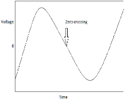
In case of discrete time signals, a zero crossing is said to occur if there is a sign difference between successive samples. The zero crossing rates (ZCR) are a simple measure of the frequency content of a signal. For narrow band signals, the average zero crossing rate gives a reasonable way to estimate the frequency content of the signal. But for a broad band signal such as speech, it is much less accurate [11]. However, by using a representation based on the short time average zero crossing rate, rough estimates of spectral properties can be obtained [3].In this expression, each pair of samples is checked to determine where zero crossings occur and then the average is computed over N consecutive samples.

(1)

Where the sgn function is

(2)

And x(n) is the time domain signal for frame m.

unvoiced sounds in the syllable rate, while music signals do not have this kind of structure. Hence, for the speech signal, variation of zero crossing rates will be in general greater than that of music signals. ZCR is a good discriminator between speech and music. Considering this, many systems have used ZCR for audio segmentation. A variation of the ZCR the high zero crossing rate ratios (HZCRR) are more discriminative than the exact value of ZCR.

Fig. 1 Zero Crossing Rate

2.1.2 Short Time Energy

Short Time Energy (STE) is used indifferent audio classification problems. In speech signals, it provides a basis for distinguishing voiced speech segments from unvoiced ones. In case of very high quality speech, the short term energy features are used to distinguish speech from silence. The energy E of a discrete time signal x(n) is defined by the expression.

(3)

The amplitude of an audio signal varies with time. A convenient representation that reflects these amplitude variations is the short time energy of the signal. In general, the short time energy is defined as follows.

(4)

The above expression can be rewritten as

(5)

Where h(m) = w2(m). The term h(m) is interpreted as the impulse response of a linear filter. The choice of the impulse response, h(n)determines the nature of the short time energy representation. Short time energy of the audible sound is in general significantly higher than that of silence segments. In some of the systems, the Root Mean Square (RMS) of the amplitude is used as a feature for segmentation. It can be used as the measurement to distinguish audible sounds from silence when the SNR (signal to noise ratio)is high and its change pattern over time may reveal the rhythm and periodicity properties of sound. These are the major reasons for using STE in segmenting audio streams of various sounds and categories [12].

2.2 Frequency Domain Features

2.2.1 Spectral Centroid

The spectral centroid is a measure used in digital signal processing to characterize a spectrum. It indicates where the “center of mass” of the spectrum is. Perceptually, it has a robust connection with the impression of “brightness” of a sound. It is calculated as the weighted mean of the frequencies present in the signal, which is determined using a Fourier transform, with their magnitudes as the weights

(6)

Where x(n) represents the weighted frequency value, or magnitude, of bin number n, and f(n) represents the center frequency of that bin.

Some people use “spectral centroid” to refer to the median of the spectrum. This is a different statistic, the difference being essentially the same as the difference between unweight median and mean statistics. Since both are measures of central tendency, in some situations they will exhibit some similarity of behavior. But since typical audio spectra are not normally distributed, the two measures will often give strongly different values. Grey and Gordon in 1978 found the mean a better fit than the median.

Because the spectral centroid is a good predictor of the “brightness” of a sound, it is widely used in digital audio and music processing as an automatic measure of musical timbre.

2.2.2 Spectral Flux

Spectrum flux (SF) is defined as the average variation value of spectrum between two adjacent frames in a given clip. In general, speech signals are composed of alternating voiced sounds and unvoiced sounds in the syllable rate, while music signals do not have this kind of structure. Hence, for speech signal, its spectrum flux will be in general greater than that of music. The spectrum flux of environmental sounds is among the highest, and changes more dramatically than those of speech and music. This feature is especially useful for discriminating some strong periodicity environment sounds such as tone signal, from music signals. Spectrum flux is a good feature to discriminate among speech, environment sound and music.

(7)

Where A(n,k) is the discrete Fourier transform of the nth frame of input signal.

(8)

2.2.3 Spectral Roll off

As the Spectral Centroid, the Spectral Roll off is also a representation of the spectral shape of a sound and they are strongly correlated. It’s defined as the frequency where85% of the energy in the spectrum is belowthat frequency. If K is thebin that fulfills

(9)

Then the Spectral Roll off frequency is f(K), where x(n)representsthe magnitude of bin number n, and f(n) representsthe center frequencyof that bin.

2.2.4 Spectral Entropy

The spectral entropy is the quantitativemeasure of thespectral disorder. The entropy has been used to detectsilence and voiced region of speech in voice activity detection.The discriminatory property of this feature gives rise to itsuse in speech recognition. The entropy can be used to capture theformants or the peakness of a distribution. Formants and their locationshave been considered to be important for speechtracking[14].

(10)

3.

CLASSIFICATION MODEL

3.1 Support VectorMachine

In machine learning, support vector machines (SVMs, also calledsupport vector networks) are supervised learning models with associatedlearning algorithms that analyze data and recognize patterns,used for classification and regression analysis. The basicSVM takes a set of input data and predicts, for each given input,which of two possible classes forms the output, making it a non-probabilisticbinary linear classifier [9],[4]. Given a set of trainingexamples, each marked asbelonging to one of two categories, an SVM trainingalgorithm builds a model that assigns new examplesinto one category or the other. An SVM model is a representationof the examples as points in space, mapped so that the examples ofthe separate categories are divided by a clear gap that is as wide aspossible. New examples are then mapped into that same space andpredicted to belong to a category based on which side of the gapthey fall on [10]. In addition to performing linear classification, SVMs can efficientlyperform non-linear classification using what is called the kerneltrick, implicitly mapping their inputs into high-dimensional featurespaces [6].

Kernel methods have received major attention, particularly due to the increased popularity of the Support Vector Machines. Kernel functions can be used in many applications as they provide a simple bridge from linearity to non-linearity for algorithms which can be expressed in terms of dot products. Some common Kernel functions include the linear kernel, the polynomial kernel and the Gaussian kernel. Below is a list of some kernel functions

3.1.1 Gaussian Kernel

The Gaussian kernel is an example of radial basis function kernel.

(11)

Alternatively, it could also be implemented using

(12)

The adjustable parameter sigma plays a major role in the performance of the kernel and should be carefully tuned to the problem at hand. If overestimated, the exponential will behave almost linearly and the higher-dimensional projection will start to lose its non-linear power. In the other hand, if underestimated, the function will lack regularization and the decision boundary will be highly sensitive to noise in training data.

3.1.2 Sigmoidal kernel

Sigmoidalkernel functions which aren’t strictly positive definite also have been shown to perform very well in practice. Despite its wide use, it is not positive semi-definite for certain values of its parameters.

(13)

wherexi is support vectors, β0, β1 are constant values.

3.1.3 Polynomial Kernel

The Polynomial kernel is a non-stationary kernel. Polynomial kernels are well suited for problems where all the training data is normalized.

(14)

Adjustable parameters are the slope alpha, the constant term c and the polynomial degree d.

4.

IMPLEMENTATION

Fig. 2 Block Diagram for speech/music classification.

4.1 Signal Pre-processing

Audio signal has to be preprocessed before extractingfeatures.There is no added information in the difference of two channelsthat can be used for classification orsegmentation. Therefore it isdesirable to have a mono signal to simplify later processes. The algorithmchecks the number of channels of the audio. If the signalhas more than one channel, it is mixed down to mono [13].

the overall amplitudelevel might have on the featureextraction [5].

4.2 Feature Extraction

Six set of features is extracted from each frame of the audio by usingthe feature extraction techniques. Here the low level featuresboth time domain and frequency domain features are taken. Thetime domain features are ZCR and STE, thefrequency domain featuresare spectral centroid, spectral flux, spectral roll-off and spectralentropy. An input wav file isgiven to the feature extractiontechniques. Six set of feature values will be calculated for the givenwav file. The above process is continued for 100 number of wavfiles. The six set of feature values for all the wav files will be storedseparately for speech and music. The features are then often normalizedby the computed mean value and the standard variationover a larger time unit and then stored in a feature vector [1].

4.3 Classification

When the feature extraction process is done the audio shouldbeclassified either as speech or music. In a more complexsystemmore classes can be defined, such as silence or speech over music.The latter is often classed as speech in systems with only two basicclasses. The extracted feature vector is used to classify whether theaudio is speech or music. A mean vector is calculated for the wholeaudio and it is comparedeither to results from training data or topredefined thresholds. A method where the classification is basedon the output of many frames together is proposed [15][7].

In this method, based on the output the feature values areextractedfrom the speech/music wav file and it is appendedwith two categories.One category is appended for speech wav and the othercategory is appended for the music wav. By using the feature valueswith appended value SVM training is carried out. As a resultof the training data two model files will be created one for speechand the other for music. The SVM trains the audio data and createtwo models one for speech and the other for music. For testing thefeatureextraction is done on different speech and music wav filesother than the speech and music wav files used in the trainingset.All the values would be used for testing, the SVMtests the featuresbased on models created during the training. Eachsecond consistsof 100 frames, and each frame is assigned a class by a SVMclassifier.Then, a global decision is made based on the most frequentlyappearing class within thatsecond.

5. RESULTS AND DISCUSSION

For classification, the audio files other than the files used fortrainingare tested. The extracted feature vector is used toclassifywhether the audio is speech or music. A mean vectoris calculatedfor the whole audio and is then compared eitherto results fromtraining data or to predefined thresholds. Amethod where the classificationis based on the output ofmany frames together is proposed.Each second consists of100 frames, and each frame is assigneda class by a SVMclassifier. The SVM will train the audiodata and create twomodules correspondingly.

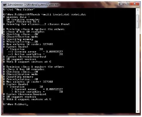
The following fig. 3 and 4 shows the SVM train and test.

Fig. 3 SVM train for Audio samples.

The training samples are loaded and two classes are created, foreach category. The two categories will be trained with twoclass 0 and class 1 with 100 examples.

Fig. 4 SVM test for Audio samples.

The testing sample is tested using the trained model and create a result. The result will show whether the audio is speech or music.

Table 1 Classification Performance for different kernel function

Kernel function Speech Music

Gaussian 85% 88%

Sigmoidal 82% 84%

Polynomial 83% 80%

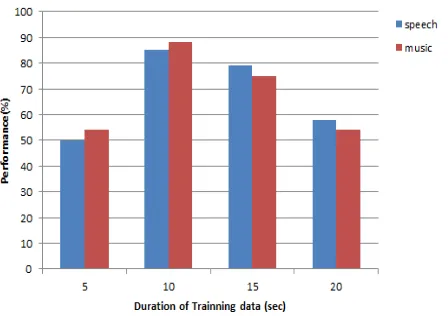
Fig. 5 Performance of audio classification for different duration of speech and music clips.

6. CONCLUSION

The system classifies the audio data into speech or music. It is currently the state of the art approach for categorization. Inorder toclassify the audio first the feature extraction is doneusing both thelow level feature time domain and frequencydomain feature. Thetime domain features are ZCR and STE,the frequency domain featuresare spectral centroid, spectralflux, spectral roll-off and spectralentropy. After featureextraction classification process is doneusing the SVM. TheSVM classifier trains the feature vectors tocreate models forclasses. The SVM test the input audio data basedon themodels created by the SVMtrain and produce the result data.Based on the result data the input audio is classified intospeech ormusic.

7. REFERENCES

[1] Boser E. Bernhard, Guyon M. Isabelle, and Vapnik N. Vladimir. A training algorithm for optimal margin classifiers. In 5th Annual ACM Workshop on COLT, pages 144–152. ACM Press, 1992.

[2] J. Breebaart and M. McKinney. Features for audioclassification. Int.Conf. on MIR, 2003.

[3] ] F. Gouyon, F. Pachet, and O. Delerue. Classifyingpercussive sounds: a matter of zero crossing rate. Proceedings of the COST G-6 Conference on DigitalAudio Effects (DAFX-00), December 2000. Verona, Italy.

[4] Hongchen Jiang, JunmeiBai, Shuwu Zhang, and Bo Xu.Svm-based audio scene classification. Proc. IEEE IntConf. Natural Lang. Processing and Knowledge Engineering, pages 131–136, October 2005.

[5] B. Liang, H. Yanli, L. Songyang, C. Jianyun, and W.Lingda. Feature analysis and extraction for audio automatic classification, Proc. IEEE Int. Conf. Systems, pages 767–772, October 2005.

[6] Lim and Chang. Enhancing support vector machine-based speech/music classification using conditional maximum a posteriori criterion. Signal Processing, IET, 6(4):335–340, June 2012.

[7] Lie Lu, Hong-Jiang Zhang, and Stan Z. Li. Content-based audio classification and segmentation by using

support vector machines,.Springer-Verlag Multimedia Systems. 8:482–492, February 2003.

[8] Ingo Mierswa1 and Katharina Morik. Automatic feature extraction for classifying audio data,.Machine Learning Journal, 58(2):127–149, February 2005.

[9] Chungsoo Lim Mokpo, Yeon-Woo Lee, and Joon-Hyuk Chang. New techniques for improving the practicality of ansvm-based speech/music classifier. Acoustics, Speech and Signal Processing (ICASSP), pages 1657–1660, March 2012.

[10]S. Nilufar, Edmonton, N. Molla, and K. Hirose. Spectrogram based features selection using multiple kernel learning for speech/music discrimination. kernel learning for speech/music discrimination. Acoustics, Speech and Signal Processing (ICASSP), pages 501–504, March 2012.

[11]C. Panagiotakis and G. Tziritas. A speech/music discriminator based on rms and zero-crossings,.IEEE Trans. Multimedia, 7(5):155–156, February 2005. [12]G. Peeters. A large set of audio features for sound

description. tech. rep., IRCAM, 2004.

[13]L. Rabiner and R.W. Schafer. Digital processing of speech signals. Pearson Education, 2005.

[14]Toru Taniguchi, MikioTohyama, and Katsuhiko Shirai. Detection of speech and music based on spectral tracking. Speech Communication, 50:547–563, April 2008.

[15]ChangshengXu, C. Namunu, Maddage, and Xi Shao. Automatic music classification and summarization. IEEE Trans. Speech and Audio Processing, 13(3):441–450, May 2005.

Authors Profile

R. Thiruvengatanadhan received his Bachelor's degree in Computer Science and Engineering from Annamalai University, Chidambaram in the year 2004. He received his M.E degree in Computer Science and Engineering from Annamalai University, Chidambaram. He is pursuing his Ph.D in Computer Science and Engineering from Annamalai University, Chidambaram. He joined the services of Annamalai University in the year 2006 as a faculty member and is presently serving as Assistant Professor in the Department of Computer Science &Engg. His research interests include audio signal processing, speech processing, image processing and pattern classification.

guiding several students who are pursuing doctoral research. Her research interests include speech processing, image and video processing, pattern classification and neural networks.

P.Suresh Kumar received his Bachelor's degree in Computer Science and Engineering from Annamalai University,Chidambaram in the year 2011. He is pursuing his