http://dx.doi.org/10.4236/ojs.2015.55047
Implementation of the Estimating Functions
Approach in Asset Returns Volatility
Forecasting Using First Order
Asymmetric GARCH Models
Timothy Ndonye Mutunga, Ali Salim Islam, Luke Akong’o Orawo
Department of Mathematics, Egerton University, Egerton, Kenya
Email: [email protected], [email protected], [email protected]
Received 26 June 2015; accepted 16 August 2015; published 19 August 2015 Copyright © 2015 by authors and Scientific Research Publishing Inc.
This work is licensed under the Creative Commons Attribution International License (CC BY).
http://creativecommons.org/licenses/by/4.0/
Abstract
This paper implements the method of estimating functions (EF) in the modelling and forecasting of financial returns volatility. This estimation approach incorporates higher order moments which are common in most financial time series, into modelling, leading to a substantial gain of infor- mation and overall efficiency benefits. The two models considered in this paper provide a better in-sample-fit under the estimating functions approach relative to the traditional maximum likely- hood estimation (MLE) approach when fitted to empirical time series. On this ground, the EF ap-proach is employed in the first order EGARCH and GJR-GARCH models to forecast the volatility of two market indices from the USA and Japanese stock markets. The loss functions, mean square error (MSE) and mean absolute error (MAE), have been utilized in evaluating the predictive ability of the EGARCH vis-à-vis the GJR-GARCH model.
Keywords
Estimating Function, Asymmetric GARCH, Volatility, Mean Square Error, Mean Absolute Error
1. Introduction
Asset return volatility is an imperative factor in pricing of derivatives and portfolio allocation in the financial world. As a result, many conventional methods for measuring the risk associated with financial assets are done through studies on the variance (volatility) of the asset price [1]. Volatility is considered as a measure of risk which is used by investors as a premium for investing in risky assets and therefore an efficient model for fore-casting an asset’s price volatility is a crucial ingredient in financial decision making.
in explaining the dynamics of return volatility in the financial markets. This has led to their extensive applica-tion to modelling and forecasting stock market returns volatility, in developed economies [2]-[5] as well as in emerging markets [6]-[10].
Consequently, much attention has been paid to the estimation of this class of models in a bid to provide an ef-ficient framework for modelling and forecasting return volatility. Different approaches among them, the maxi-mum likelihood (ML), the estimating functions (EF) and the Bayesian adaptive Markov chain Monte Carlo (MCMC) methods, have been utilized in estimation of the symmetric/asymmetric GARCH models and volatility prediction [11]-[13]. An efficient estimation method translates to an improved predictive ability of the model. The ultimate goal of volatility analysis must be to explain the causes and predict future volatility values.
The focus of this paper is to implement the method of estimating functions based on [14]’s optimal estimating functions for stochastic processes, in the asset return volatility prediction in the Asymmetric GARCH family of models. First order EGARCH and GJR-GARCH models estimated in [13] are utilised in forecasting asset return volatility of empirical time series from the USA and Japanese stock markets. A brief overview of the first order EGARCH and GJR-GARCH models is presented in Section 2. Optimal estimating functions for the Asymmetric GARCH—class of models in general and the first order EGARCH and GJR-GARCH models are presented in Section 3. Forecast ability of the two first order Asymmetric GARCH models is evaluated in Section 4. Finally, a conclusion of this paper is presented in Section 5.
2. GARCH Models with Asymmetry
There is extensive empirical evidence that stock returns exhibit asymmetric volatility, that is, there is existence of asymmetric effects of positive and negative past returns on volatility [15]-[18]. To model this aspect, this pa-per considers two of the most popular asymmetric GARCH models.
2.1. EGARCH Model
The EGARCH model by [19] addresses some of the key limitations of the conventional GARCH model. This model captures asymmetric responses of the conditional variance to shocks in the market. The EGARCH
(
p q,)
is specified as;( )
1 1
ln ln
t t t
p q
t i t i i t i
i i
z h
h h g z
ε
κ β − α −
= = = = + +
∑
∑
(1)where, α1=1,εt =zt ht, g z
( )
t =γ1zt+γ2zt −E zt .The model specifies the variance equation as the log of the variance series hence the leverage effect is exponential and therefore the parameters κ β, i andαi are not restricted to be non-negative. αi is the asymmetry parameter.
The quantity g z
( )
t is a function of both magnitude and sign of zt in order to accommodate theasymmet-ric effect [19]. The components γ1ztandγ2zt −E zt represent the sign effect and magnitude effect respec-tively and each has a zero mean.
Over the range 0<zt < ∞, g z
( )
t is linear in zt with slope γ γ1+ 2 while over the range −∞ <zt<0,( )
tg z is linear in zt with slope γ γ1− 2. Thus g z
( )
t allows the conditional variance ht to respondasym-metrically to changes in stock returns.
2.2. GJR-GARCH Model
The GJR-GARCH model was introduced by [20]. It is a variant of the GARCH model with the ability to capture asymmetries between positive and negative shocks of the same magnitude on the volatility of returns. The vari-ance equation in GJR-GARCH
(
p q,)
model is specified as;(
2 2)
1 1
1 when 0 0 otherwise
t t t
p q
t i t i t i t i i t i
i i
t t
z h
h s h
s
ε
κ α ε γ ε β
ε − − − − − = = − = = + + + < =
where, zt ~iid N 0,1
( )
.The model reduces to the traditional GARCH model whenever ε ≥t 0. The indicator term st
−
captures the asymmetric effect of past returns on current volatility. With γ >0, negative shocks
(
εt−1<0)
increase vola-tility more than positive shocks(
εt−1>0)
of equal magnitude. The necessary and sufficient conditions to guarantee positivity of the conditional variance ht are κ >0,α >0,β>0 andα γ+ >0. γ is the asymmetryparameter.
3. Estimation of the Asymmetric GARCH Models Using Estimating Functions
In this section we state some important results on estimating functions for the asymmetric GARCH models. [13] derived the optimal estimating functions for the Asymmetric Garch family of models, based on the works of [21] and [14]. The optimal EFs as presented in [13] are given in (3)
(
)
(
)
*
1 2
1 2 1
1 2 1 * 2 2 2 1 1 2 2 1 1 2 2 t T
t t t t
t t t
T
t
t t
T t t
t t t t t t
h
g
h
x x h
h g
h h
θ λ
φ φ
ω φ ω
ω λ ω ωλ
φ φ = = = ∂ ∂ = − + − ∂ ∂ ∂ − ∂ ∂ ∂ = − + − +
∑
∑
∑
(3)where, ht is the conditional variance process given in (1) and (2). The estimates for the unknown parameter
vectors ω and θ are obtained by solving the optimal EFs in (3) by numerically minimising g1 g2
∗+ ∗
. First order EGARCH and GJR-GARCH models have been fitted to the Standard and Poor’s 500 and the Nik-kei 225 market indices for the period 2nd Jan 2008 to 31st May 2011. The estimated models under the EFs ap-proach are presented in (4), (5), (6) and (7).
S&P 500 index
1 1 1 1
lnht = −0.204886 0.976205 ln+ ht− +0.138098zt− −0.161534zt− −E zt− (4)
2 2
1 1 1 1
2.37614E 06 0.00113883 0.16956 0.902273
t t t t t
h = − + ε− + s−−ε− + h− (5)
Nikkei 225 index
1 1 1 1
lnht= −0.285148 0.966433ln+ ht− +0.147311zt− −0.147345zt− −E zt− (6)
2 2
1 1 1 1
1.0501E 05 0.00618129 0.185744 0.857417
t t t t t
h = − + ε− + s−−ε− + h− (7)
where,
t t t z h ε
= and 1 when 0
0 otherwise
t t
s− = ε <
.
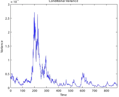
[image:3.595.212.417.537.704.2]The time plots of the estimated conditional variance series in (4), (5), (6) and (7) are given inFigures 1-4 re-spectively.
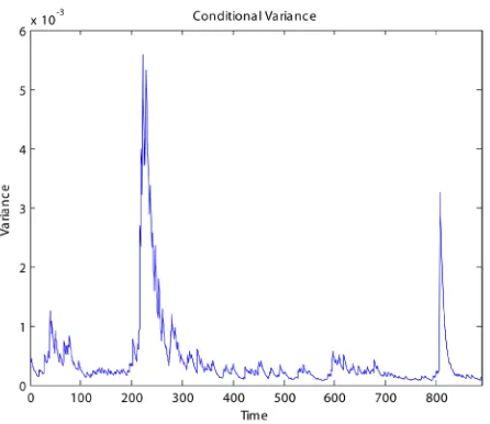
Figure 2. Time plot of the estimated conditional variance in (5).
Figure 3. Time plot of the estimated conditional variance in (6).
[image:4.595.204.427.508.701.2]The time plots inFigures 1-4 indicate that the estimated conditional variance is extremely high for some pe-riods and relatively low in others (time variant) which is a common feature in most financial data.
4. Forecasting the Volatility of Financial Asset Returns of the USA and Japan Stock
Markets
The fitted models under the EF approach have been used for forecasting the daily volatility of stock returns for the S&P 500 index and Nikkei 225 index data sets. Out-of-Sample forecasting is performed for the period (1st June 2011 to 13th October 2012).
Forecasts for the first order EGARCH and GJR-GARCH conditional variance processes over m = 500 days (future time horizon) have been generated. Given the log conditional variance process lnh1, lnh2, lnh3,, lnhn
for the EGARCH and conditional variance process h h h1, 2, 3,,hn for the GJR-GARCH model, predictions for
1 2 3
lnhn+, lnhn+ , lnhn+ ,, lnhn m+ and hn+1,hn+2,hn+3,,hn m+ have been generated for the forecast period m =
500.
The conditional variance ht is time varying (volatile) and is the object of interest in the forecasting process.
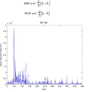
In the case that only daily closing prices are available, the daily squared returns is an appropriate proxy for the unobserved volatility that fully accounts for the time varying property. The daily squared returns have for long and widely been used as a proxy of the latent realized variance [22]. In this study, the daily squared returns over the forecast period have been used as a proxy for the unobserved variance which is incorporated in the loss functions used to generate the error statistics used for evaluating the predictive ability of the two first order asymmetric GARCH models.
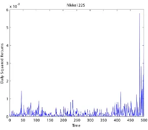
The time plots of the daily squared returns over the forecast period m=500, for the two data sets are given inFigure 5 andFigure 6.
The following two loss functions have been used to evaluate the out-of-sample forecast performance of the models. They include the Mean Square Error (MSE) and the Mean Absolute Error (MAE).
(
)
21
1 MSE
m
t t
t
m− h h
=
=
∑
− (8) 1
1 MAE
m
t t
t
m− h h
=
[image:5.595.170.526.389.705.2]=
∑
− (9)Figure 6. Time plot of the daily squared returns for the Nikkei 225 index.
where, mis the number of days in the out-of-sample period, ht is the proxy of the actual volatility and ht is the volatility forecast at day t. The loss functions have been used to compute forecasts errors of the models.
Table 1 presents the forecasts error statistics used to evaluate the forecast performance of the models.
The forecast ht at time t is used in computing the forecast ht+1 at time t+1, for t=1, 2,,m due to the recursive nature of these models. It is observed that as the forecasts are generated recursively, the recursion converges asymptotically to the theoretical unconditional variance of the processes.
For the EGARCH (1,1) process the unconditional variance is given in (10).
2 1 ε
κ σ
β
= −
(10)
For the GJR-GARCH (1,1) process the unconditional variance is given in (11).
2
1 1
2 ε
κ σ
α β γ
=
− − −
(11)
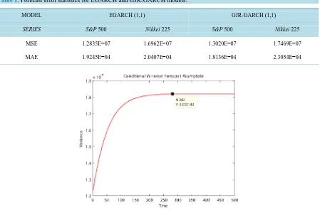
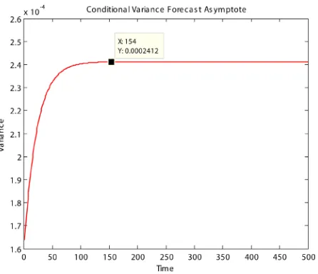
Time plots of the conditional variance forecast asymptotes for the two models and data sets are given in Fig-ures 7-10.
Figure 7 andFigure 8 present the conditional variance forecast asymptotes of the two models for the S&P 500 index data set. Figure 9 and Figure 10 present the conditional variance forecast asymptotes of the two models for the Nikkei 225 index data set.
It is observed that for the S&P 500 index, the volatility forecasts converge asymptotically to the unconditional variance (0.000182, 0.0002003) after about (282, 263) data points for the EGARCH (1,1) and GJR-GARCH (1,1) processes respectively. For the Nikkei 225 index, the volatility forecasts converge asymptotically to the uncon-ditional variance (0.0002045, 0.0002412) after about (216, 154) data points for the EGARCH (1,1) and GJR- GARCH (1,1) processes respectively.
Discussion
model that is preferred based on both loss functions as mixed results are obtained across the two data sets (see
Table 1). However considering the MSE, the first order EGARCH model provides the best out-of-sample vola-tility forecast than the GJR-GARCH model. The more robust loss function, MAE indicates that the first order GJR-GARCH model performs better but for only one data set, S&P 500 index. Thus the ranking of models in terms of forecast performance based on a specific loss function varies across the two data sets over the consid-ered forecast period. This inconsistency in ranking stresses the importance of selecting an adequate loss function for forecasting purposes. The two models forecast a general increase in conditional variance before the proc-esses converge to the theoretical unconditional variances.Figure 8 andFigure 10 show that the first order GJR- GARCH process forecasts converge faster to the unconditional variance than the corresponding EGARCH process forecasts (seeFigure 7 andFigure 9) implying that the latter process has a higher forecast memory.
5. Conclusion
In this paper the main objective was to implement the method of optimal estimating functions in volatility esti-mation and prediction using Asymmetric GARCH modes. First order EGARCH and GJR-GARCH models have then been used in forecasting asset volatility of the USA and Japan stock markets using the S&P 500 and Nikkei 225 indices respectively under the EF approach. The two models have recorded mixed out-of-sample forecast performance results across the data sets. However the MSE and MAE statistics are generally lower for the EGARCH model across the two data sets except for a single case where the GJR-GARCH model records a lower MAE for the S&P 500 index data set. Thus first order EGARCH model performed relatively better than the first order GJR-GARCH model in forecasting volatility over the considered forecast period.
Acknowledgements
This research paper was prepared and made possible through the help and support of my academic supervisors, The German Academic Exchange Service (DAAD) and the African Mathematics Millennium Science Initiative
Table 1. Forecast error statistics for EGARCH and GJR-GARCH models.
MODEL EGARCH (1,1) GJR-GARCH (1,1)
SERIES S&P 500 Nikkei 225 S&P 500 Nikkei 225
MSE 1.2835E−07 1.6962E−07 1.3020E−07 1.7469E−07
[image:7.595.91.540.408.703.2]MAE 1.9245E−04 2.0407E−04 1.8136E−04 2.3054E−04
Figure 8. Time plot of the GJR-GARCH (1,1) conditional variance forecast asymptote.
Figure 9. Time plot of the EGARCH (1,1) conditional variance forecast asymptote.
[image:8.595.204.427.511.703.2](AMMSI) who sponsored my postgraduate studies.
References
[1] Lars, K.M. (2002) GARCH-Modelling: Theoretical Survey, Model Implementation and Robustness Analysis. Masters Thesis, Royal Institute of Technology (KTH), Stockholm.
[2] Bollerslev, T., Chou, R. and Kroner, K.F. (1992) ARCH Modelling in Finance: A Review of the Theory and Empirical Evidence. Journal of Econometrics, 52, 5-59. http://dx.doi.org/10.1016/0304-4076(92)90064-X
[3] Chappel, D., Padmore, J. and Pidgeon, J. (1998) A Note on ERM Membership and the Efficiency of the London Stock Exchange. Applied Economics Letters, 5, 19-23. http://dx.doi.org/10.1080/758540120
[4] Janne, K. (2012) GARCH models for Foreign Exchange Rates. Bachelors Thesis, Aalto University, Aalto.
[5] Li, Y. (2013) GARCH Models for Forecasting Volatilities of Three Major Stock Indicies Using Both Frequentist and Bayesian Approach. Masters Thesis, Ball State University, Muncie, IN.
[6] Su, D. and Fleisher, B.M. (1998) Risk, Return and Regulation in Chinese Stock Markets. Journal of Economics and
Business, 50, 239-256. http://dx.doi.org/10.1016/S0148-6195(98)00002-2
[7] Kalu, O.E. (2010) Modelling Stock Returns Volatility in Nigeria Using GARCH Models. MPRA (Munich Personal RePEc Archive) Paper No. 23432.
[8] Olweny, T. (2011) Modelling Volatility of Short-term Interest Rates in Kenya. International Journal of Business and
Social Science, 2, 289-303.
[9] Suliman, Z.S. and Peter, W. (2012) Modelling Stock Market Volatility using Univariate GARCH Models: Evidence from Sudan and Egypt. International Journal of Economics and Finance, 4, 161-176.
[10] Wagalla, A., Nassiuma, D.K., Islam, A.S. and Mwangi, J.W. (2012) Volatility Modelling of the Nairobi Stock Ex-change Returns Using the ARCH-Type Models. International Journal of Applied Science and Technology, 2, 165-174.
[11] Mwangi, J.W. (2007) Parameter Estimation for Nonlinear Time Series Models Using Estimating Functions. PhD The-sis, Egerton University, Kenya.
[12] Neelabh, R. (2009) Conditional Heteroscedastic Time Series Models with Asymmetry and Structural Breaks. PhD Thesis, University of Pune, Pune.
[13] Mutunga, T.N., Islam, A.S. and Orawo, L.A. (2014) Estimation of Asymmetric GARCH Models: The Estimating Functions Approach. International Journal of Applied Science and Technology, 4, 198-209.
[14] Godambe, V.P. and Thompson, M.E. (1989) An Extension of the Quasi-Likelihood Estimation. Journal of Statistical
Planning and Inference, 22, 137-172. http://dx.doi.org/10.1016/0378-3758(89)90106-7
[15] Black, F. (1976) Studies of Stock Price Volatility Changes. Proceedings of the 1976 Meetings of the American Statis-tical Association, Business and Economics Statistics Section, Boston, 25-26 August 1976, 177-181.
[16] Engle, R.F. and Ng, V.K. (1993) Measuring and Testing the Impact of News on Volatility. Journal of Finance, 48, 1749-1778. http://dx.doi.org/10.1111/j.1540-6261.1993.tb05127.x
[17] Wu, G. (2001) The Determinants of Asymmetric Volatility. Review of Financial Studies, 14,837-859. http://dx.doi.org/10.1093/rfs/14.3.837
[18] Blair, B., Poon, S. and Taylor, S.J. (2002) Asymmetric and Crash Effects in Stock Volatility for the S&P 100 Index and Its Constituents. Applied Financial Economics, 12, 319-329. http://dx.doi.org/10.1080/09603100110090154
[19] Nelson, D.B. (1991) Conditional Heteroskedasticity in Asset Returns: A New Approach. Econometrica, 59, 347-370. http://dx.doi.org/10.2307/2938260
[20] Glosten, L.R., Jagannathan, R. and Runkle, D. (1993) On the Relation between the Expected Value and the Volatility of Nominal Excess Returns on Stocks. Journal of Finance, 48, 1779-1801.
http://dx.doi.org/10.1111/j.1540-6261.1993.tb05128.x
[21] Godambe, V.P. (1960) An Optimum Property of Regular Maximum Likelihood Equations. Annals of Mathematical
Statistics, 31, 1208-1211. http://dx.doi.org/10.1214/aoms/1177705693