Skmer: assembly free and alignment free sample identification using genome skims

M E T H O D

Open Access

Skmer: assembly-free and alignment-free

sample identification using genome skims

Shahab Sarmashghi

, Kristine Bohmann

, M. Thomas P. Gilbert

, Vineet Bafna

and Siavash Mirarab

Abstract

The ability to inexpensively describe taxonomic diversity is critical in this era of rapid climate and biodiversity changes. The recent genome-skimming approach extends current barcoding practices beyond short markers by applying low-pass sequencing and recovering whole organelle genomes computationally. This approach discards the nuclear DNA, which constitutes the vast majority of the data. In contrast, we suggest using all unassembled reads. We introduce an assembly-free and alignment-free tool, Skmer, to compute genomic distances between the query and reference genome skims. Skmer shows excellent accuracy in estimating distances and identifying the closest match in reference datasets.

Keywords: Assembly-free, Alignment-free, DNA Barcoding, Genome skimming, DNA reference database, Second generation sequencing

Background

The ability to quickly and inexpensively study the taxo-nomic diversity in an environment is critical in this era of rapid climate and biodiversity changes. The current molecular technique of choice is (meta)barcoding [1–3]. Traditional (meta)barcoding is based on DNA sequenc-ing of taxonomically informative and group-specific marker genes (e.g., mitochondrial COI [1,4] and 12S/16S [5,6] for animals, chloroplast genes like matK for plants [7], and ITS [8] for fungi) that are variable enough for taxonomic identification, but have flanking regions that are sufficiently conserved to allow for PCR amplification using universal primers. Barcoding is used for taxonomic identification of single-species samples. In the case of metabarcoding, the goal is to deconstruct the taxonomic composition of a mixed sample consisting of multiple species [3]. Beyond the barcoding application, the barcod-ing marker genes have also been used to delimitate species [9] and to infer phylogenies [10,11].

The accuracy of (meta)barcoding depends on the cov-erage of the reference database and the method used to

*Correspondence:[email protected];[email protected]

1_{Department of Electrical & Computer Engineering, University of California,} San Diego, La Jolla, CA 92093, USA

5_{Department of Computer Science & Engineering, University of California, San} Diego, La Jolla, CA 92093, USA

Full list of author information is available at the end of the article

search queries against it [3]. To increase coverage, ref-erence databases with millions of barcodes have been generated (e.g., Barcode of Life Data System, BOLD, for COI [12]). Computational methods for finding the clos-est match in a reference dataset (e.g., TaxI [13]), and for placement of a query into existing marker trees [14–16] have been developed. However, the traditional approach to (meta)barcoding, despite its success, has some draw-backs. PCR for marker gene amplification requires rela-tively high-quality DNA and thus cannot be applied to samples in which the DNA is heavily fragmented. More-over, since barcode markers are relatively short regions, their phylogenetic signal and identification resolution can be limited [17]. For example, in a recent study, 896 out of 4,174 wasp species could not be distinguished from each other using COI barcodes [18].

While low costs have kept PCR-based pipelines attrac-tive, decreasing costs of shotgun sequencing have now made it possible to shotgun sequence 1–2 Gb of total DNA per reference specimen sample for as low as $80 [19], even after including sample preparation and labor costs. This has lead researchers to propose an alter-nate method that uses low-pass sequencing to generate genome skims[19,20], and subsequently identifies chloro-plast or mitochondrial marker genes or assembles the organelle genome. Reconstructing plastid and mtDNA genomes from low-pass shotgun data is possible because

organelle DNA tends to be heavily overrepresented in shotgun sequencing data; for example, 10.4% of all reads from the Apocynaceae family of flowering plants were from the chloroplast in one genome-skimming study [20]. Large reference databases based on genome-skimming techniques are under construction by projects such as PhyloAlps [21], NorBol [22], and DNAmark [23].

Most current applications of genome skimming to species identification require organelle genome assem-bly, a task that requires relatively time-consuming manual curation steps to ensure that assembly errors are avoided [24]. This approach discards a vast proportion of the non-target data, reducing the discriminatory power. For these reasons, the DNAmark project [23] is consider-ing alternative methods, where, instead of only relyconsider-ing on organelle markers, one could use the entire set of reads generated in a genome skim as the identifier of a species. This approach poses an interesting method-ological question: can the unassembled data be used to taxonomically profile reference and query samples in a similar manner to conventional barcoding, but using all available genomic information and saving us from the labor-intensive task of mitochondria/plastid genome assembly? In this paper, we introduce a new assembly-free method to directly use low-coverage genome skims of both reference and query samples. By avoiding the assembly step, our approach also reduces the amount of data processing needed for expanding the reference database.

We treat genome skims simply as low-coverage “bags of reads,” both for a collection of reference species and for query samples. The problem is to find the refer-ence genome skim that matches the query; if an exact match is not found, we seek the closest available match. A more advanced problem, not directly addressed here, is placing the query in a phylogeny of reference species. An even more difficult challenge, also not addressed here, is decomposing a query genome skim that con-tains DNA from several different taxa into its constituent species.

Central to solving these problems is the ability to esti-mate adistancebetween two genome skims for low and varied coverage using assembly-free and alignment-free approaches. Alignment-free sequence comparison has been widely studied [25–30], including for phylogenetic reconstruction [25,31–44]. Most existing methods, such as Kr [28], spaced words [44], and kmacs [45], compute evolutionary distances using the length distribution of matched substrings or the count of certain words and thus require assembled genomes to produce accurate results. These methods will not work with high accuracy when both the query and the reference are a set of reads and not assembled contigs. Other methods, such as andi [41] and FSWM [43], use micro-alignments to compute distances.

Even though it may be possible to extend the idea of using micro-alignments to the assembly-free case, both andi and FSWM software currently require assemblies as input. However, several assembly-free methods also exist. Co-phylog [39] makes micro-alignments and calculates distances to reconstruct phylogenetic trees; Mash [46] computes the Jaccard index and an evolutionary distance using the k-mers; Simka [47] computes several distance measures based on the whole k-mer content of reads. However, these methods all assume high enough cover-age, ensuring that most of the genome is covered. These levels of coverage are currently not economically feasible for building up large reference databases or for obtaining many query samples. Among existing methods, AAF [33] is the only one that aims to work even at lower coverage. AAF first infers a phylogeny and then corrects its branch lengths to reflect a given estimate of the coverage.

Here, we show that high levels of coverage are not nec-essary. We focus on a distance measure defined as the pro-portion of mismatches between the global alignment of two genomes. The mismatch rate, called genomic distance hereafter, is useful for species identification because it reflects the evolutionary divergence between two species. We introduce a new method, Skmer, for accurately com-puting the genomic distance even from low-coverage genome skims. In extensive test, we show that Skmer dra-matically improves estimates of genomic distance based on genome skims and accurately places genome-skim queries on to a reference collection. This assembly-free approach can therefore be considered a viable comple-ment to currently available DNA barcoding and genome-skimming tools.

Results Skmer

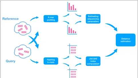
We decomposed reads into fixed-length oligomers (denotedk-merswith lengthk), a technique used by many existing alignment-free methods [41,48]. Recall that the Jaccard index J is a similarity measure between any two sets (e.g., k-mer collections) defined as the size of their intersection divided by the size of their union. Ondov et al. describe a tool, Mash [46], in which (a) J is esti-mated efficiently using a hashing procedure and (b) J is used to estimate the genomic distance between two genomes. Mash, however, assumes sufficiently high cov-erage. Unfortunately, J, in addition to the true distance, is impacted by coverage, sequencing error, and genome length. Skmer accounts for the impact of these factors onJ. Skmer has two stages (Fig. 1): first, we usek-mer fre-quency profiles (computed using JellyFish [49]) to esti-mate the amount of sequencing error and the coverage (neither of which is known) using a novel method. LetMi

Fig. 1Overview of Skmer pipeline. For both query and reference genome skims, first, the k-mer frequency profiles are used to estimate the sequencing error and coverage (top). Then, the k-mers are hashed, and a subset is retained and used to estimate the Jaccard index between the two genomes (bottom). Finally, the estimated Jaccard index and estimated sequencing coverage and error are used to compute the corrected genomic distance between the query and the reference

we derive (see “Estimating sequencing coverage and error rate” section):

λ= M1

Mh ξh

h!e

−ξ_+ξ1−e−ξ ₍₁₎

=1−(ξ/λ)1/k (2)

whereλandare our estimates of thek-mer coverage and the sequencing error rate, respectively.

In stage two, we use the hashing technique of Mash to computeJ. Finally, given these estimates, we compute the genomic distance using

D=1−

2(ζ1L1+ζ2L2)J

η1η2(L1+L2)(1+J)

1/k

(3)

where fori ∈ {1, 2},ηi = 1−e−λi(1−i) k

andζi = ηi+ λi

1−(1−i)k

(for high coverage, we defineζi andηi

differently; see “Sequencing error” section for details), and Liis the estimated genome length.

We used a series of experiments to study the accuracy of Skmer compared to existing methods with respect to (i) the error in computed distances, (ii) the ability to find the closest match to a query sequence in a reference dataset of genome skims, and (iii) phylogenetic inference. We com-pared the performance againstMashandAAF[33]. AAF

is a method that uses k-mers to estimate phylogenetic distances among a set of at least four sequences. We con-clude by comparing Skmer against the results of using COI barcodes from available barcode databases.

Distance accuracy for pairs of genome skims

We first compare the accuracy of Mash and Skmer in esti-mating distances between two genome skims. Since AAF outputs a phylogenetic tree and so requires at least four species, we cannot include it in our first set of analyses on pairs of genomes.

Simulated genomes with controlled distance

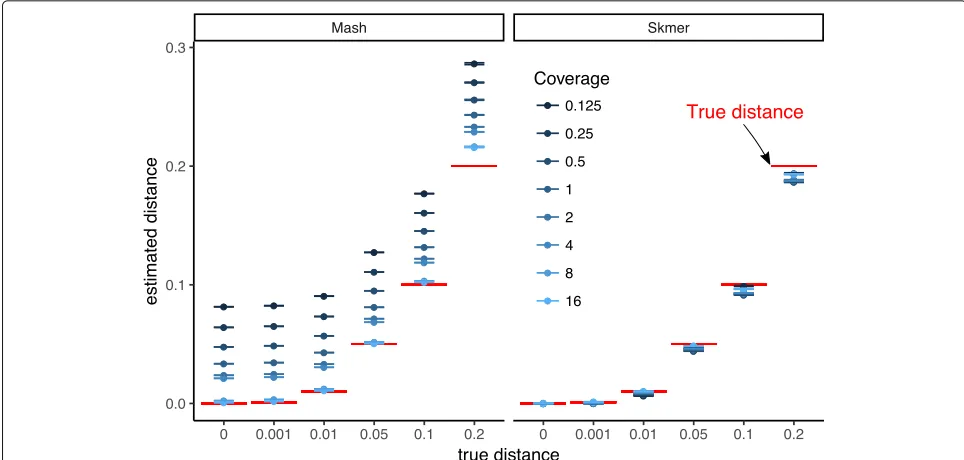
Fig. 2Comparing the accuracy of Mash and Skmer on simulated genomes. Genome skims are simulated using ART with read length=100. Substitutions applied to the assembly ofC. vestalisat six different rates (x-axis), and genome skims simulated at varying coverage range from1₈to 16×. The estimated distance (y-axis) by Mash (left) and Skmer (right) is plotted versus the real distances for each coverage level (color). The mean (dots) and standard error (lines) of distances are shown (10 repeats). True distance is shown in red. See Additional file1: Figure S1 for a scaled representation

distance to 0.045 (an underestimation by 10%). Note that applying Mash* (Mash without the unnecessary approx-imation (1− D)k ≈ e−kD used by default in Mash) to the complete assemblies generally generates very accu-rate results, as expected, but even given the full assembly, Mash* still has a small but noticeable error whend=0.2. Note that results are extremely consistent across our ten different runs of subsampling (Fig. 2). We repeated the simulation with a lower range of coverage (₆₄1×to 1×). Interestingly, even with very low coverage, the absolute distance error is small in many cases (Additional file1: Figure S2); however, ford≥0.1, Skmer estimates start to degrade below 1₈×coverage.

Repeating the process with theDrosophila melanogaster genome as the base genome also produces similar results (Additional file 1: Figure S3). The only condi-tion where Skmer has an absolute error larger than 0.01 is with coverage below 1× and d = 0.2 (Fig. 2). However, we note that for d = 0.001, the rela-tive error is not small with low coverage (Additional file 1: Figure S4b) indicating that distinguishing very small distances (perhaps below species level) requires high coverage. Estimating the right order of magnitude when the true distance is 0.001 seems to require 2× coverage (preferably 8×) while 1× coverage is sufficient to distinguish distances at or above 0.01 (Additional file1: Figure S4).

Pairs of insect and bird genomes

We now test methods on several pairs of insect and avian genomes, subsampled to create genome skims. Note that unlike the simulated datasets, here, genomes can undergo all types of genetic variations and complex rearrange-ments, and thus, do not have the same length. We carefully selected several pairs of genomes to cover a wide range of mutation distance and genome length.

Here, the true genomic distance is not known, but we use the distance estimated by Mash* on the full assem-blies as the true distance d. For all pairs of insect and avian genomes (Fig. 3), Mash has high error for cov-erage below 8× while Skmer successfully corrects the estimated distance and obtains values extremely close to the results of running Mash* on the full assembly. For example, the distance betweenAnopheles stephensi with length of∼196 Mbp andAnopheles maculatuswith length of∼132 Mbp is estimated to be 0.104 based on the full assembly and 0.102 (2% underestimation) with only 1₂× coverage using Skmer, while Mash would estimate the distance to be 0.163 (∼57% overestimation).

Distance accuracy for all pairs genome skims

a

b

Fixed sequencing effort

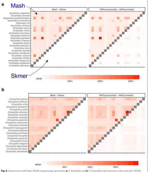
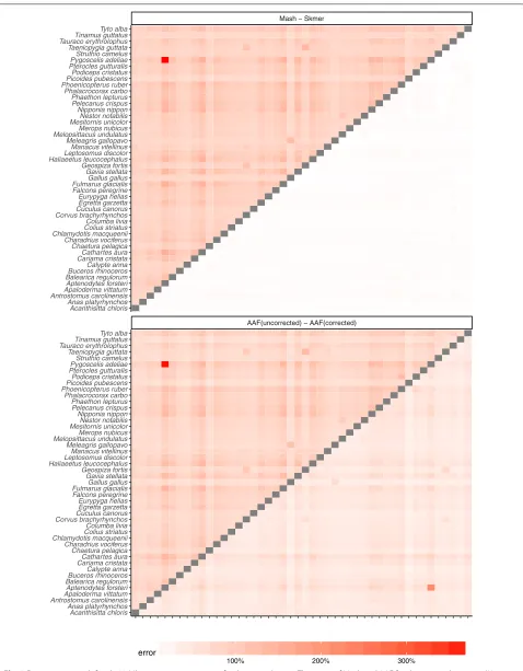
So far, our experiments have controlled for the coverage by subsampling varying amounts of sequence data, pro-portional to the genome length. In our genome-skimming application, coverage will not be fixed. Often, the amount of sequence data obtained for each species will be rel-atively similar. As a result, genomes of different length end up being sequenced with different coverage depth proportional to the inverse of their length. We therefore performed a study where all species are subsampled to produce 100 Mb of sequence data in total resulting in varying levels of coverage (based on the genome length, Additional file1: Table S5). The error in the distance esti-mated by Mash relative to the ground truth can be quite large (higher than 300% in the worst case) while Skmer consistently makes accurate estimates close to the true distance even at the lowest amount of coverage (Figs. 4 and5, and Additional file1: Table S6). Repeating the anal-ysis with 0.5 Gb or 1 Gb total sequence data produced similar patterns, but as expected, increasing the sequenc-ing effort reduces the error for all methods (Additional file1: Figures S6-S8).

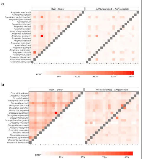
Before error correction, AAF has error levels that are comparable to Mash (Figs.4, 5). The correction applied by AAF, similar to Skmer, reduces the negative impact of low coverage but not to the same extent. Thus, Skmer has less error compared to corrected AAF (with 100 Mb sequence and across all datasets, the mean error of Skmer is 3.13% and AAF-corrected is 22.7%). For example, in the Drosophiladataset, the worst-case error of AAF between any two pairs of genome skims is 31%, whereas the error never exceeds 8% for Skmer. Note that when computing the error of AAF, we use the result of running AAF on full assemblies as the ground truth.

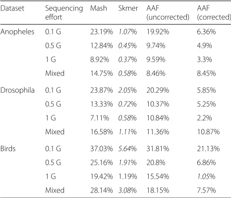
To quantify the impact of distance estimates on down-stream analyses, we used FastME [50] to infer phyloge-netic trees using distances computed by Mash and Skmer on genome skims and with correction using the JC69 model [51]. AAF by default generates trees as part of its output. We compare these trees to those computed by Mash/AAF run on the full assemblies (taken as the ground truth) using the weighted Roubinson-Foulds (WRF) dis-tance [52] (Table1). WRF is the sum of branch length differences between the two trees (using zero length for missing branches), and we normalized WRF by the sum of branch lengths of both trees. In all three datasets, Skmer distances lead to trees with lower WRF distance to the ground truth compared to Mash and AAF/uncorrected. AAF correction reduces WRF compared to uncorrected AAF; however, Skmer trees have two to 14 times less error compared to the corrected AAF, except in one case where AAF/corrected has 1.05% error and Skmer has 1.19% (Table1). Increasing the size of skims to 0.5 Gb and 1 Gb helps all methods to produce more accurate trees.

Heterogeneous sequencing effort

In addition to changes in the genomic length, the sequenc-ing effort per species may also vary across sequencsequenc-ing pro-tocols, experiments, and research labs, and so a database of reference genome skims may consist of samples with heterogeneous sequencing efforts. To capture this, for each species, we choose its total sequencing effort from three possible values 0.1 Gb, 0.5 Gb, and 1 Gb, uniformly at random, and estimate all pairs of distances within each dataset as before (Fig.6and Additional file1: Figure S9). Similar to the case of fixed sequencing effort, Skmer mit-igates large relative error in the distances estimated by Mash and produces more accurate results than both Mash and AAF (Table2, Fig.6, and Additional file1: Figure S9). For example, comparing to the case of fixed 100-Mb genome skims of theDrosophila dataset, the worst-case error of AAF is increased to 70%, while using Skmer it remains almost the same (8%). Comparing trees inferred from distances estimated by various methods also con-firms the higher accuracy of Skmer (Table1). For instance, on the Anopheles dataset, Skmer has only 0.58% WRF distance to the reference tree whereas Mash and AAF-corrected trees have 14.75% and 8.45% WRF distance.

Genome skims from real reads Running time

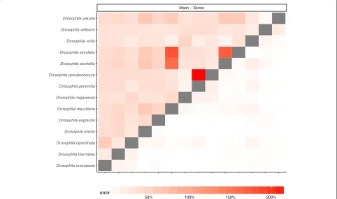
So far, all of our tests used simulated reads. When analyz-ing real genome skims, there are additional complications such as extraneous DNA (real or artifactual) and the over-representation of organelle genome. We next tested Skmer using real reads. We created 100-Mb skims of 14 Drosophila genomes by subsampling short-read data produced in a recent Drosophila genome assembly study [53]. Before running Skmer or Mash, we filtered reads that (even partially) aligned to 12 Drosophila-associated microbial genomes as reported in previous studies [54–56] (see Additional file 1: Table S1), to the human genome, or to the mitochondrial genome of respective Drosophila species. We then estimated all pairs of dis-tances as before and computed the error relative to the distances computed from the assemblies (Fig.7). Consis-tent with the results that, we obtained on the simulated skims, Skmer has less error compared to Mash. The aver-age error of Mash on this dataset is 43.48% (±2.29%) with maximum error of 217%. Skmer, on the other hand, has an average error of 4.21% (±0.35%) and its maximum error is 22.2%.

Skmer and Mash have comparable running time, while AAF is much slower. In the experiment with heterogeneous sequencing effort, the total running time (using 24 CPU cores) to compute distances based

on genome skims for all

47 2

pairs of birds using

a

b

Fig. 4Distance error with fixed 100 Mb sequence per genome fora22 Anopheles andb21 Drosophila. Each genome is skimmed with 100 Mb sequence and distances are computed using Mash, Skmer, and AAF. True distance used in calculating the error is computed by applying each method (AAF and Mash) to the full genome assemblies. The heatmaps on the left show the error of Mash (upper triangle) and Skmer (lower triangle), and the heatmaps on the right are for AAF before correction (upper) and after correction (lower)

Leave-out search against a reference database of genome skims We now study the effectiveness of using genomic dis-tance to search a database of genome skims to find the

Table 1Tree error

Dataset Sequencing

effort

Mash Skmer AAF

(uncorrected) AAF (corrected)

Anopheles 0.1 G 23.19% 1.07% 19.92% 6.36%

0.5 G 12.84% 0.45% 9.74% 4.9%

1 G 8.92% 0.37% 9.59% 3.3%

Mixed 14.75% 0.58% 8.46% 8.45%

Drosophila 0.1 G 23.87% 2.05% 20.29% 5.85%

0.5 G 13.33% 0.72% 10.37% 5.25%

1 G 7.11% 0.58% 10.84% 2.2%

Mixed 16.58% 1.11% 11.36% 10.87%

Birds 0.1 G 37.03% 5.64% 31.81% 21.13%

0.5 G 25.16% 1.91% 20.8% 6.86%

1 G 19.42% 1.19% 15.54% 1.05%

Mixed 28.14% 3.08% 18.15% 7.57%

For each method, we show normalized weighted RF distance (%) of trees inferred from genome-skim distances to trees inferred from full assembly distances. Italics: the lowest error

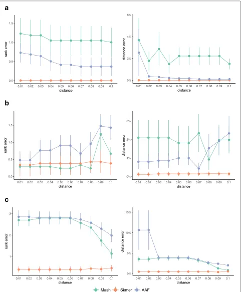
the query. The results can be provided to the user as a ranking. When the query genome is available in the refer-ence dataset, finding the match is relatively easy. To study the effectiveness of the search as the distance of the closest available match increases, we use a leave-out experiment, as described in “Leave-out” section. Figure8 shows the mean rank error as well as the mean distance error of the best remaining match in a leave-out experiment when removing genomes closer thandfor 0.01 ≤ d ≤ 0.1. A rank error (or distance error) equal to zero corresponds to a perfect match to the best available genome.

On all three datasets, Skmer consistently and often sub-stantially outperforms Mash and AAF in terms of finding the best remaining match, except theDrosophiladataset where Mash and Skmer have comparable rank error, while both are better than AAF (Fig.8). Even in that case, on average, the distance of the best match found by Skmer is closer to the distance of the true best match compared to the best hit found by Mash. Moreover, the mean rank error of Skmer is smaller than Mash (Additional file 1: Figure S10) if we exclude only one species Drosophila willistoni(which is at distance 0.1565≤d≤0.1622 from other species). It is also notable that over the avian dataset, Skmer has mean rank error less than 0.5 for all range of distances, while Mash and AAF can be off by more than 2.5 on average. These results demonstrate that correcting the distance not only impacts our understanding of the absolute distance, but also impacts results of searching a reference library.

Phylogeny reconstruction and comparison to organelle markers As the last experiment, we estimated phylogenetic trees forAnophelesandDrosophiladatasets after transforming

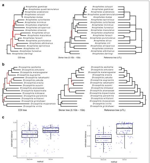
the genomic distances estimated by Skmer to Jukes-Cantor (JC) distances [51]. For each dataset, we also built another tree based on available COI barcodes, using an identical method. We compare the results against a ref-erence tree obtained from Open Tree of Life [57]. We restricted the results to species for which COI barcodes were available (Fig.9ab).

For theAnopheles species, Skmer distances produce a tree that is almost identical to the reference tree (with only one branch difference out of nine), while COI tree dif-fers from the reference in seven branches. Similarly, for theDrosophilaspecies, Skmer differs from the reference in three branches (with small local changes) out of 13 total branches in the reference tree, whereas COI tree is very inconsistent with the reference tree (seven branches are different). We also built maximum-likelihood trees from COI barcodes (Additional file1: Figure S11), but the num-ber of incorrect branches did not reduce. Comparing the distribution of all pairwise genomic distances obtained from genome skims and barcodes (Fig. 9c), Skmer has larger distances and fewer pairs with zero or close to zero distance, indicating that Skmer has a higher resolution in differentiating between samples. For example, four species of the Anophelesgenus A. coluzzii, A. gambiae, A. ara-biensis, andA. melashave very small pairwise distances based on COI barcodes, while using Skmer, the estimated distances are in the range 0.02–0.04 for these species.

Discussion

We showed that Skmer can compute the genomic dis-tance between a pair of species from genome skims with very low coverage (at or even below 1×), with much bet-ter accuracy than the main two albet-ternatives, Mash and AAF. We also showed that the distances computed by Skmer can accurately place a voucher genome skim within a reference database of genome skims, and can be used to infer the phylogenetic tree with reasonable accuracy. While Skmer is not the first k-mer-based approach for distance estimation or phylogenetic reconstruction, as we showed, the alternatives have low accuracy given low-coverage data. We compare with Mash because it is used within Skmer and is one of the most widely used align-ment and assembly-free methods. However, we note that authors of Mash do not claim it can handle low coverage, and so our results are not a criticism of their approach. Besides the methods we discussed, many other alignment-free sequence comparison and phylogeny reconstruction algorithms exist [25, 28, 29, 31, 32, 34–43]. However, these methods take as input assembled (but unaligned) sequences, and thus, are not applicable in an assembly-free pipeline. In other words, their goal is to avoid the alignment step and not the assembly step.

a

b

Fig. 6Distance error with heterogeneous sequencing effort foraAnopheles andbDrosophila. Species have random amount of sequence chosen uniformly among 0.1 Gb, 0.5 Gb, and 1 Gb. See Additional file1: Figure S9 for birds

from the nuclear genome, improves the phylogenetic accuracy. These improvements are resulting from dis-tances that have a larger range and more resolution compared to COI. Also, the increased resolution should

Table 2Comparing the average error of Mash, Skmer, and AAF in estimating distances over three datasets with heterogeneous sequencing effort

Dataset Mash Skmer AAF

(uncorrected) AAF (corrected)

Anopheles 28.72% (1.10%) 0.84% (0.03%) 13.48% (0.56%)

11.36% (0.44%)

Drosophila 29.05% (0.59%) 0.84% (0.04%) 15.25% (0.38%)

10.94% (0.33%)

Birds 64.29% (0.54%) 2.21% (0.04%) 36.02% (0.29%)

5.28% (0.16%)

The standard error of the mean is provided in parentheses. Italics: the lowest error

that can further reduce the accuracy of marker genes for both species identification and phylogeny reconstruc-tion. By using the entire genome, Skmer ensures that an average distance across the genome is computed, reduc-ing the sensitivity to gene tree/species tree discordances. Moreover, a recent result shows that the JC-transformed genomic distance is a statistically consistent estimator of the species distances despite gene tree discordance due to incomplete lineage sorting [59], further encouraging our use of the genomic distance as a measure of the evolutionary divergence.

We showed that genomic distances as small as 0.01 can be estimated accurately from genome skims with 1×

or lower coverage. What does a distance of 0.01 mean? The answer will depend on the organisms of interest. For example, two eagle species of the same genus ( Hali-aeetus albicillaandHaliaeetus leucocephalus) haveD ≈ 0.003 but two Anopheles species of the same species complex (A. gambiaeand A. coluzzii) have D ≈ 0.018. Broadly speaking, for eukaryotes, detecting distances in the 10−2 order is often enough to distinguish between species (Additional file1: Figure S12). On the other hand, to differentiate individuals in a population, or very sim-ilar species, we may need to reliably estimate distances of the order 10−3. Detection at these lower levels seems to require> 1×coverage using Skmer (Additional file1: Figure S4b) but future work should study the exact level of sequencing required for accurate ordering of species at distances in the order of 10−3 _{or less. Moreover, the}

question of the minimum coverage required may avail itself to information-theoretical bounds and near-optimal solutions, similar to those established for the assembly problem [60,61].

Although most of our tests were performed on genome skims simulated from assemblies, we also tested Skmer on genome skims simulated by subsampling previous whole-genome sequencing experiments. Several compli-cations have to be addressed in real applicompli-cations. The actual coverage of real genome skims may not be uniform

a

b

c

a

b

c

Fig. 9Comparing distances and phylogenetic trees from COI barcodes and simulated genome skims. Shown in red are wrong internal branches corresponding to the bipartitions that are not found in the reference tree. Genome-skim size is randomly chosen among 0.1 Gb, 0.5 Gb, and 1 Gb. aAnophelestrees.bDrosophilatrees.cDistribution of distances forAnopheles(left) andDrosophila(right) genomes

and randomly distributed and they can have an overrep-resentation of mitochondrial or plastid sequence. More importantly, other sources of DNA originating from for example, parasites, diet, fungi, commensals, bacteria, and human contamination may all be present in the sample

sufficient to produce reliable distance estimates in the case of Drosophila genomes. We recommend that before using Skmer, such database searches should be used to find and eliminate bacterial or fungal contamination (using BLAST [62] or perhaps metagenomic tools such as Kraken [63]), as well as removing contaminant reads with human ori-gin (using for example Bowtie2 [64]). However, in future, it will be beneficial to develop better methods for finding extraneous reads without reliance on known sources.

A related direction of future work is to explore whether Skmer can be extended to environmental DNA analyses, i.e., queries consisting of genome skims of multi-taxa sam-ples. While Skmer is presented here in a general setting, its best use is for eukaryotic organisms, where the notion of species is better established and species can be sepa-rated with reasonable effort. We tested Skmer on birds and insects, but we predict it will work equally well for plants, a prediction that we plan to test in future work.

Throughout our experiments, we used Mash* run on the assemblies to compute the ground truth. Given the true alignment of the two genomes, we can compute the true genomic distance as the proportion of mismatches among aligned orthologous positions (i.e., ignoring gaps). To ensure that Mash* closely approximates true distances, we used simulated genomes of Rat and Mouse from the Mam-malian dataset of the Alignathon competition [65]. This simulation uses Evolver [66] and includes many forms of mutation, including indels, rearrangements, duplications, and losses. On this dataset, the true distance based on the known true alignment is 0.145 and Mash* estimated the distance as 0.143, which is a very good approximation. In contrast, FastANI [67], an alignment-free sequence mapping tool for estimating average nucleotide identity, computes the distance as 0.189. If we count gaps as non-matching positions in the definition of distance, then the true distance would be 0.287, which also does not match FastANI. Presumably, FastANI, which relies on alignment of short blocks, counts short gaps (with somedefinition of short) as mismatch but excludes larger ones. Thus, on real data, Mash* is the best available option to approxi-mate the true distance. Finally, note that, for real genomes, we chose not to use estimated whole genome alignments (WGA) to compute the ground truth because WGA is a difficult problem, and WGAs that are available are not necessarily accurate. We get inconsistent estimates of dis-tance when we use pairwise or multiple WGAs. For exam-ple, betweenD. melanogasterandD. yakuba, the distance changes from 0.10 when using the multiple WGA [68], to 0.21 if we use the pairwise WGAs [69] from the UCSC genome browser [70], which is the state of the art.

The connection between genomic distance and phy-logenetic distance depends on mutation processes con-sidered. If only substitutions are allowed and assum-ing the Jukes-Cantor model, the phylogenetic distance

is−3₄ln1− 4₃d; note this transformation is monotonic and does not change rankings of matches to a query search. Assuming a more complex model such as GTR [71], genomic distance is not enough to estimate the phy-logenetic distance. However, we have devised a simple procedure to estimate GTR distances using the log-det approach [72] by repeated applications of Skmer to per-turbed reads (Additional file 1: Appendix B). The GTR distances can rank matches to a query differently from the genomic distance; the accuracy of the two distances should be compared in future work.

Insertions, deletions, duplications, and losses can all lead to differences between genomes, thereby reducing the Jaccard index and increasing the genomic distance. They also impact genomic length. Interestingly, in our experiments, Skmer run with the true coverage is less accurate than with estimated coverage (Additional file1: Figure S13). We speculate that on genomes with repeats, by overestimating coverage, our method gives an estimate of the “effective” coverage, reducing the impact of repeats on the Jaccard index. Nevertheless, with these complex mutations, the correct definitions of the evolutionary dis-tance and genomic disdis-tance are not straightforward, nor is it clear how the Jaccard index should be translated to the genomic distance. Here, we used a heuristic approach that simply averaged the length of the two genomes, leav-ing these broader questions about the best definition of genomic distance in the presence of large structural vari-ations to future work.

Conclusions

Skmer is an assembly-free and alignment-free tool for esti-mating the distance between two genome skims. It can estimate a wide range of distances with high accuracy from low-coverage and mixed-coverage genome skims with no prior knowledge of the coverage or the sequenc-ing error. Our paper shows that the idea of genome-wide sample identification using genome skims has merit and should be pursued in the future.

Methods

Throughout, we present our results succinctly and present derivations and more careful justifications in Additional file1: Appendix A of the supplementary material.

Jaccard index versus genomic distance

The Jaccard index of subsetsA1andA2is defined as

J= |A1∩A2|

|A1∪A2| =

|A1∩A2|

|A1| + |A2| − |A1∩A2|

. (4)

Let W be the number of shared k-mers between the two genomes. Note thatJ = _2LW_−W ⇒ ₁2₊J_J = W_L, where Lis the genome length. Assuming random genomes and no repeats, perhaps justifiably [73], the probability that a changedk-mer exists elsewhere in the genome is van-ishingly small for sufficiently largek. Thus, we assume a k-mer is in the sharedk-mers set only if no mutation falls on it, an event that has probability(1−d)k. Thus, we can modelW as a binomial with probability(1−d)k andL trials. As Ondov et al. [46] pointed out, we can estimate

D=1−

2J J+1

1

k

(5)

and they further approximate D as 1_klnJ+_2J1. To be able to estimate large distances, we avoid the unneces-sary approximation and use Eq.5directly. We skim each genome to obtaink-mer setsA1,A2and estimateJusing

Eq.4, which can be computed efficiently using a hashing technique used by Mash [46]. Note that, however, Eq.5 assumes a high coverage of the genome so that eachk-mer is sampled at least once with very high probability. This assumption is violated for genome skims in consequential ways. As a simple example, suppose the coverage is low enough that ak-mer is sampled with probability 0.5. Then, even for identical genomes, we estimateJ as 1₃, resulting in a distance estimate ofD≈0.032 fork=21.

Extending to genome skims with known low coverage and error

We now show how Eq.5can be refined to handle genome skims despite low and uneven coverage, sequencing error, and varying genome lengths. We first assume that cover-age and error are known and later show how to compute these.

Low coverage

When the genome is not fully covered, three sources of randomness are at work: mutations and sampling of k-mers from each of the two genomes. Each genome of lengthLis sequenced independently using randomly dis-tributed short reads of length at coverages c1 andc2

to produce two genome skims. Under the simplifying assumption that genomes are not repetitive, we choose k to be large enough so that eachk-mer is unique with high probability. Therefore, the number of distinctk-mers

in each genome isL−k L. The probability of cover-ing eachk-mer can be approximated asηi = 1− e−λi

whereλi=ci(1−k/). Modeling the sampling ofk-mers

as independent Bernoulli trials,|Ai|becomes binomially

distributed with parametersηi andL. By independence, W = |A1∩A2|also becomes binomially distributed with

parametersη1η2(1−d)kandL. Moreover,U= |A1∪A2|

can also be modeled approximately as a Gaussian with meanη1+η2−η1η2(1−d)k

L. Treating η1 and η2 as

known and dividingW_L byU_L gives us:

J= W

U =

η1η2(1−D)k

η1+η2−η1η2(1−D)k

;

thus,

D=1−

_(η

1+η2)

η1η2

J (1+J)

1

k .

Sequencing error

Each error reduces the number of shared k-mers and increases the total number of observedk-mers, and thus can also change the Jaccard index. Letidenote the

base-miscall rate for genome skimi. For largekand smalli, the

probability that an erroneousk-mer produces a non-novel k-mer is negligible. The probability that ak-mer is covered by at least one read, without any error, is approximately

ηi=1−e−λi(1−i) k

. (6)

Adding up the number of error-free and erroneous k-mers, the total number of k-mers observed from both genomes can again be approximately modeled as a Gaussian with meanζiLfor

ζi=ηi+λi

1−(1−i)k

. (7)

Just as before, we can simply estimateDby solving for it in

J= η1η2(1−D) k

ζ1+ζ2−η1η2(1−D)k

. (8)

When the coverage is sufficiently high, eachk-mer will be covered by multiple reads with high probability, and low-abundancek-mers can be safely considered as erro-neous. Mash has an option to filter out k-mers with abundances less than some thresholdmto removek-mers that are likely to be erroneous. In this case,

ζi=ηi=1− mi−1

t=0

λi(1−i)k t

t! e

−λi(1−i)k ₍₉₎

assuming all erroneousk-mers are removed. For instance, filtering single-copyk-mers (i.e.,m=2) gives us:

ζi=ηi=1−e−λi(1−i) k

−λi(1−i)ke−λi(1−i) k

we filter low-coverage k-mers only when our estimated coverage is higher than a threshold (described below). Note that the genome skims compared may use different filtering schemes, yet Eq.8holds regardless.

Differing genome lengths

Based on a model where the genomic distance between genomes of different lengths is defined to be confined to the mutations that are falling on homologous sequences, we can drive

J= η1η2min(L1,L2)(1−D) k

ζ1L1+ζ2L2−η1η2min(L1,L2)(1−D)k

.

This computation does not penalize for genome length difference. While a rigorous modeling of evolutionary distance for genomes of different length requires sophis-ticated models of gene gain, duplication, and loss, we take the heuristic approach used by Ondov et al. [46] and sim-ply replace min(L1,L2) with (L1 + L2)/2. This ensures

that the estimated distance increases as genome lengths becomes successively more different. This leads us to our final estimate of distance given by:

D=1−

2(ζ1L1+ζ2L2)J

η1η2(L1+L2)(1+J)

1/k

(10)

Estimating sequencing coverage and error rate

So far we have assumed a perfect knowledge of sequencing depth and error. However, for genome skims, the genome length is not known; thus, we need to estimate the cov-erage in order to apply our distance correction. We also assume a constant base error rate, and co-estimate it with the coverage.

The sequencing depth, which is the average number of reads covering a position in the genome, can be esti-mated from thek-mer coverage profiles. The probability distribution of the number of reads covering ak-mer is a Poisson r.v. with meanλ, whereλis defined ask-mer cov-erage. As we look into the histogram data, it is easier to work with counts instead of probabilities. LetMdenote the total number of k-mers of length k in the genome, andMi count the number ofk-mers covered byi reads.

Thus, for i ≥ 0, E[Mi]= Mλ i

i!e−λ. For a given set of

reads, we can count the number of times that eachk-mer is seen, and assuming zero sequencing error, it equals the number of reads covering thatk-mer. Then, we can aggre-gate the number of k-mers covered by i reads and find Mi fori ≥ 1. However, since in a genome skim, large

parts of the genome may not be covered, bothMandM0

are unknown. To deal with this issue, we could take the ratio of consecutive counts to get a series of estimates of λ as λ˜i = M_Mi+_i1(i+ 1) for i = 1, 2,. . .. In practice,

sequencing errors change the frequency ofk-mers and has

to be considered when estimating the coverage. Assum-ing that the error is introduced at a constant rate along the reads, we can use the information in the k-mer counts to co-estimate andλ. Like before, we assume that the k-mer lengthkis large enough that any error will intro-duce a novelk-mer, so the count of all erroneousk-mers is added to the count of single-copyk-mers. Moreover, for k-mers with more than one copy, the number of times that eachk-mer is seen equals the number of reads covering thatk-mer without any error. Formally, letMˆidenote the

count ofk-mers seenitimes in the presence of error, and ρ=(1−)kdenote the probability of error-freek-mer.

E Mˆi

= j≥iMλ j j!e−λ

_j i

ρi_(1−ρ)j−i _i≥2

j≥1Mλ

j j!e−λ

jρ(1−ρ)j−1+j(1−ρ) i=1

=

Mξ_i!ie−ξ i≥2 Mξe−ξ+λ−ξ i=1

(11)

whereξ = λρ is the average number of error-free reads covering ak-mer. A family of estimates forξ is obtained by taking the ratio of consecutive counts of error-freek -mers asξ˜i= Mˆ_Mˆi+1

i (i+1)fori≥2. Then, using an estimate ofξ and the count of single-copyk-mers, we get a series of estimates ofλfori≥2 as

˜

λi=

ˆ M1 ˆ Mi ˜ ξi i!e

−˜ξ_{+ ˜ξ1−e}−˜ξ _{. (12)}

Moreover, we can estimate the error rate from the esti-mates ofλandξas

˜

=1−

˜

ξ/λ˜1/k . (13)

While any of these ξ˜i andλ˜i can be used in principle,

the empirical performance can be affected by the choice; in our tool, we use heuristic rules (described below) that seek to use largeMivalues.

Skmer: implementation

Skmer takes as input two or more genome skims. It uses JellyFish [49] to computeMivalues, which are then used

in estimatingλandbased on Eqs.12and13, by setting

˜

ξ = ˜ξhandλ˜ = ˜λh, whereh=argmaxi≥2Mi. Then, Mash

is used to estimate the Jaccard index, withk=31 (selected empirically; Additional file1: Figure S14) and sketch size 107_{. Finally, we use Eq.10to compute the hamming}

Experimental setup Method settings

For Skmer, we use the default parameters described above. For Mash, similar to Skmer, we used k = 31 (selected empirically; Additional file1: Figure S14) and sketch size 107. As Mash handles errors by removing low copy k -mers, we set the minimum cardinality for k-mers to be included asc₅+1 with our estimate ofc.

AFF has an algorithm to correct hamming distances for low coverage, but the correction relies on adjusting the length of tip branches in a distance-based inferred phy-logeny. As such, it cannot run on a pair of genomes and requires at least four genomes. Also, AAF leaves cover-age estimation to the user with some guidelines, which we fully follow (Additional file1: Appendix C).

For building phylogenetic trees, we transformed Skmer distances using the JC69 [51] model and used FastME [50] to construct the distance-based trees via BIONJ [74] method.

Genomic datasets

We used an assembly ofCotesia vestalis(GenBank acces-sion: GCA_000956155.1) as well as three sets of publicly available assembled genomes (Additional file 1: Tables S2-S4) and used ART [75] to simulate genome skims of read length=100 with default sequencing error profile, controlling for the sequencing depth (coverage) (Addi-tional file1: Appendix C). Specifically, the data included 21Drosophila genomes (flies) and 22 genomes from the Anophelesgenus (mosquitoes) obtained from InsectBase [76], and 47 avian species from the Avian Phylogenomic Project [77,78].

For the experiment on real genome skims, high-coverage SRA’s of 14 Drosophila species were obtained from NCBI database under project number PRJNA427774 [79] and then subsampled to 100 Mb. Assemblies used to compute true distances for these 14 Drosophila species were obtained from the Drosophila project [80]. We used the tool fastp [81] for filtering low-quality reads and adapter removal. We also used Megablast [82] to search against a database of bacterial and mitochondrial genomes and remove contaminant reads. We used Bowtie2 [64] with the highest sensitivity to remove the reads aligning (even partially) to the human reference genome.

To simulate genomes with controlled genomic distance, we introduced random mutations. As a challenging case, we took the highly repetitive assembly of the wasp species Cotesia vestalis, and mutated it artificially; we only applied single nucleotide mutations distributed uniformly at ran-dom across the genome. We repeated the study on the simpler case of the fly speciesD. melanogaster. We gen-erate genome skims using ART with = 100, default error profile of Illumina sequencer, and varying cover-age between ₆₄1× and 16×. For simulated genomes, we

repeated the subsampling 10 times and reported the mean and standard error.

In order to compare with DNA barcoding method, we downloaded available COI barcodes for the Drosophila andAnophelesspecies in the BOLD database [12]. Out of 21Drosophila and 22 Anopheles species in our dataset, 16 Drosophila and 19 Anopheles species had one or more barcodes in BOLD. For each species, we selected a barcode, and using MUSCLE [83], aligned all barcodes within each dataset and constructed the phylogenetic tree assuming the Jukes-Cantor model. Under the same model of substitution, we transformed Skmer distances and built the Skmer tree. We used FastME [50] to construct the distance-based trees via the BIONJ [74] method. The maximum-likelihood COI trees were built using PhyML [84].

Evaluation metrics

For simulated data, the true distance is controlled and is thus known. For biological datasets, the ground truth is unknown. Instead, we use the distance measured on the full assembly by each method as its ground truth; thus, the ground truth for AAF is computed using AAF. We show both absolute error and the relative error, measured asdˆ−_ddwhere d anddˆ are the true and the estimated distances.

Leave-out

We used a leave-out strategy to study the accuracy of searching for a query genome in a reference set. For a query genomeGqin a set ofn genomes{G1. . .Gn}, we

ordered all genomes based on their distances toGq

cal-culated using the full assemblies, which represents the ground truth; letG1_q. . .Gn_qdenote the order, andd1_q. . .dn_q be the respective distances from the query (noteG1

q=Gq

andd1_q =0). For 0.01≤ d≤ 0.10, we removed genomes 1. . .ifrom the datasets whereiis the largest value such thatdi_q≤d, leaving us withG_qi+1. . .Gn_q. We then ordered the remaining genomes by each method; letx1. . .xn−ibe

the order obtained by a method and letrbe the the rank of the best remaining genome according to the ground truth in the estimated orderi.e.,x1=Giq+r

. Sincer=1 implies perfect performance, and r > 1 indicates error, we measured rank error as the mean ofr−1 across all query genomes (1≤q≤n). Moreover, the mean (relative)

distance error is defined as the mean of d i+r q −di+q1

dqi+1 over all queries.

Additional file

Acknowledgements

We thank the reviewers for the constructive feedback.

Funding

This work was supported by the National Science Foundation (NSF) grant IIS-1815485 to SS, VB, and SM. KB was supported by the Independent Research Fund Denmark, DFF grant 5051-00140. The authors also thank the Aage V. Jensen Naturfond for financial support for the “DNAmark” project.

Availability of data and materials

Skmer software is publicly available on https://github.com/shahab-sarmashghi/Skmerunder a BSD 3-Clause license. The version of software used in the manuscript is deposited in zenodohttps://doi.org/10.5281/zenodo. 1871480[85]. The detailed description of genomic datasets used in our experiments with Skmer is provided in “Genomic datasets” section, and links for downloading the data can be found athttps://shahab-sarmashghi.github. io/Skmer/. Moreover, the GenBank accession numbers of the assemblies and the exact commands used to simulate genome skims are provided in Additional file1.

Authors’ contributions

All authors conceived the idea. SS, VB, and SM developed the algorithm. SS implemented the software and performed all experiments. All authors contributed to the analyses of data and the writing. All authors read and approved the final manuscript.

Ethics approval and consent to participate

Not applicable.

Consent for publication

Not applicable.

Competing interests

The authors declare that they have no competing interests.

Publisher’s Note

Springer Nature remains neutral with regard to jurisdictional claims in published maps and institutional affiliations.

Author details

1_{Department of Electrical & Computer Engineering, University of California,} San Diego, La Jolla, CA 92093, USA.2_{Evolutionary Genomics, Natural History} Museum of Denmark, University of Copenhagen, Copenhagen, Denmark. 3_{School of Biological Sciences, University of East Anglia, Norwich, Norfolk, UK.} 4_{Norwegian University of Science and Technology, University Museum, 7491} Trondheim, Norway.5_{Department of Computer Science & Engineering,} University of California, San Diego, La Jolla, CA 92093, USA.

Received: 4 March 2018 Accepted: 16 January 2019

References

1. Hebert PDN, Cywinska A, Ball SL, deWaard JR. Biological identifications through DNA barcodes. Proc R Soc B Biol Sci. 2003;270(1512):313–21. https://doi.org/10.1098/rspb.2002.2218.0005074v1.

2. Savolainen V, Cowan RS, Vogler AP, Roderick GK, Lane R. Towards writing the encyclopaedia of life: an introduction to DNA barcoding. Philos Trans R Soc B Biol Sci. 2005;360(1462):1805–11.https://doi.org/10. 1098/rstb.2005.1730.

3. Taberlet P, Coissac E, Pompanon F, Brochmann C, Willerslev E. Towards next-generation biodiversity assessment using DNA metabarcoding. Mol Ecol. 2012;21(8):2045–50.https://doi.org/10.1111/j.1365-294X.2012. 05470.x.

4. Seifert KA, Samson RA, deWaard JR, Houbraken J, Levesque CA, Moncalvo JM, Louis-Seize G, Hebert PDN. Prospects for fungus identification using CO1 DNA barcodes, with Penicillium as a test case. Proc Natl Acad Sci. 2007;104(10):3901–6.https://doi.org/10.1073/pnas. 0611691104.

5. Vences M, Thomas M, van der Meijden A, Chiari Y, Vieites DR. Comparative performance of the 16S rRNA gene in DNA barcoding of amphibians. Front Zool. 2005;2:5.https://doi.org/10.1186/1742-9994-2-5. 6. Ardura A, Linde AR, Moreira JC, Garcia-Vazquez E. DNA barcoding for

conservation and management of Amazonian commercial fish. Biol Conserv. 2010;143(6):1438–43.

7. Hollingsworth PM, Forrest LL, Spouge JL, Hajibabaei M, Ratnasingham S, van der Bank M, Chase MW, Cowan RS, Erickson DL, Fazekas AJ, Graham SW, James KE, Kim KJ, Kress WJ, Schneider H, van AlphenStahl J, Barrett SCH, van den Berg C, Bogarin D, Burgess KS, Cameron KM, Carine M, Chacon J, Clark A, Clarkson JJ, Conrad F, Devey DS, Ford CS, Hedderson TAJ, Hollingsworth ML, Husband BC, Kelly LJ, Kesanakurti PR, Kim JS, Kim YD, Lahaye R, Lee HL, Long DG, Madrinan S, Maurin O, Meusnier I, Newmaster SG, Park CW, Percy DM, Petersen G, Richardson JE, Salazar GA, Savolainen V, Seberg O, Wilkinson MJ, Yi DK, Little DP. A DNA barcode for land plants. Proc Natl Acad Sci. 2009;106(31):12794–7. https://doi.org/10.1073/pnas.0905845106.

8. Schoch CL, Seifert KA, Huhndorf S, Robert V, Spouge JL, Levesque CA, Chen W, Bolchacova E, Voigt K, Crous PW, Miller AN, Wingfield MJ, Aime MC, An KD, Bai FY, Barreto RW, Begerow D, Bergeron MJ, Blackwell M, Boekhout T, Bogale M, Boonyuen N, Burgaz AR, Buyck B, Cai L, Cai Q, Cardinali G, Chaverri P, Coppins BJ, Crespo A, Cubas P, Cummings C, Damm U, de Beer Z. W., de Hoog G. S., Del-Prado R, Dentinger B, Dieguez-Uribeondo J, Divakar PK, Douglas B, Duenas M, Duong TA, Eberhardt U, Edwards JE, Elshahed MS, Fliegerova K, Furtado M, Garcia MA, Ge ZW, Griffith GW, Griffiths K, Groenewald JZ, Groenewald M, Grube M, Gryzenhout M, Guo LD, Hagen F, Hambleton S, Hamelin RC, Hansen K, Harrold P, Heller G, Herrera C, Hirayama K, Hirooka Y, Ho HM, Hoffmann K, Hofstetter V, Hognabba F, Hollingsworth PM, Hong SB, Hosaka K, Houbraken J, Hughes K, Huhtinen S, Hyde KD, James T, Johnson EM, Johnson JE, Johnston PR, Jones EBG, Kelly LJ, Kirk PM, Knapp DG, Koljalg U, Kovacs GM, Kurtzman CP, Landvik S, Leavitt SD, Liggenstoffer AS, Liimatainen K, Lombard L, Luangsa-ard JJ, Lumbsch HT, Maganti H, Maharachchikumbura SSN, Martin MP, May TW, McTaggart AR, Methven AS, Meyer W, Moncalvo JM, Mongkolsamrit S, Nagy LG, Nilsson RH, Niskanen T, Nyilasi I, Okada G, Okane I, Olariaga I, Otte J, Papp T, Park D, Petkovits T, Pino-Bodas R, Quaedvlieg W, Raja HA, Redecker D, Rintoul TL, Ruibal C, Sarmiento-Ramirez JM, Schmitt I, Schussler A, Shearer C, Sotome K, Stefani FOP, Stenroos S, Stielow B, Stockinger H, Suetrong S, Suh SO, Sung GH, Suzuki M, Tanaka K, Tedersoo L, Telleria MT, Tretter E, Untereiner WA, Urbina H, Vagvolgyi C, Vialle A, Vu TD, Walther G, Wang QM, Wang Y, Weir BS, Weiss M, White MM, Xu J, Yahr R, Yang ZL, Yurkov A, Zamora JC, Zhang N, Zhuang WY, Schindel D. Nuclear ribosomal internal transcribed spacer (ITS) region as a universal DNA barcode marker for Fungi. Proc Natl Acad Sci. 2012;109(16): 6241–6.https://doi.org/10.1073/pnas.1117018109.

9. Zhang D-s, Zhou Y-d, Wang C-s, Rouse G. A new species of

Ophryotrocha (Annelida, Eunicida, Dorvilleidae) from hydrothermal vents on the Southwest Indian Ridge. ZooKeys. 2017;687:1–9.https://doi.org/ 10.3897/zookeys.687.13046.

10. Hedin MC, Maddison WP. A Combined Molecular Approach to Phylogeny of the Jumping Spider Subfamily Dendryphantinae (Araneae: Salticidae). Mol Phylogenet Evol. 2001;18(3):386–403.https://doi.org/10. 1006/mpev.2000.0883.

11. Taylor KH, Rouse GW, Messing CG. Systematics of Himerometra (Echinodermata: Crinoidea: Himerometridae) based on morphology and molecular data. Zool J Linnean Soc. 2017;181(2):342–56.

12. Ratnasingham S, Hebert PDN. BOLD : The Barcode of Life Data System (www.barcodinglife.org). Mol Ecol Notes. 2007;7(April 2016):355–64. https://doi.org/10.1111/j.1471-8286.2006.01678.x.9809069v1. 13. Steinke D, Vences M, Salzburger W, Meyer A. TaxI: a software tool for

DNA barcoding using distance methods. Philos Trans R Soc B Biol Sci. 2005;360(1462):1975–80.https://doi.org/10.1098/rstb.2005.1729. 14. Mirarab S, Nguyen N, Warnow T. SEPP: SATé-Enabled Phylogenetic

Placement. Pac Symp Biocomput. 2012;247–58.

15. Berger SA, DK, Stamatakis A, Krompass D. Performance, Accuracy, and Web Server for Evolutionary Placement of Short Sequence Reads under Maximum Likelihood. Syst Biol. 2011;60(3):291–302.https://doi.org/10. 1093/sysbio/syr010.

16. Matsen FA, Kodner RB, Armbrust EV. pplacer: linear time

17. Hickerson MJ, Meyer CP, Moritz C, Hedin M. DNA Barcoding Will Often Fail to Discover New Animal Species over Broad Parameter Space. Syst Biol. 2006;55(5):729–39.https://doi.org/10.1080/10635150600969898. 18. Quicke DLJ, Alex Smith M, Janzen DH, Hallwachs W, Fernandez-Triana J,

Laurenne NM, Zaldívar-Riverón A, Shaw MR, Broad GR, Klopfstein S, Shaw SR, Hrcek J, Hebert PDN, Miller SE, Rodriguez JJ, Whitfield JB, Sharkey MJ, Sharanowski BJ, Jussila R, Gauld ID, Chesters D, Vogler AP. Utility of the DNA barcoding gene fragment for parasitic wasp phylogeny (Hymenoptera: Ichneumonoidea): Data release and new measure of taxonomic congruence. Mol Ecol Resour. 2012;12(4):676–85.https://doi. org/10.1111/j.1755-0998.2012.03143.x.

19. Coissac E, Hollingsworth PM, Lavergne S, Taberlet P. From barcodes to genomes: extending the concept of dna barcoding. Mol Ecol. 2016;25(7): 1423–8.https://doi.org/10.1111/mec.13549.

20. Straub SCK, Parks M, Weitemier K, Fishbein M, Cronn RC, Liston A. Navigating the tip of the genomic iceberg: Next-generation sequencing for plant systematics. Am J Bot. 2012;99(2):349–64.https://doi.org/10. 3732/ajb.1100335.

21. Génomique F. Mutualisation des compétences et des équipements français pour l’analyse génomique et la bio-informatique.https://www. france-genomique.org/. Accessed 16 Oct 2018.

22. Norwegian Barcode of Life (NorBOL).http://www.norbol.org/en/. Accessed 16 Oct 2018.

23. DNAmark.http://dnamark.ku.dk/english/. Accessed 16 Oct 2018. 24. Tonti-Filippini J, Nevill PG, Dixon K, Small I. What can we do with 1000

plastid genomes?. Plant J. 2017;90(4):808–18.https://doi.org/10.1111/tpj. 13491.0608246v3.

25. Blaisdell BE. A measure of the similarity of sets of sequences not requiring sequence alignment. Proc Natl Acad Sci U S A. 1986;83(14):5155–9. 26. Vinga S, Almeida J. Alignment-free sequence comparison–a review.

Bioinformatics. 2003;19(4):513–23.https://doi.org/10.1093/ bioinformatics/btg005.

27. Zielezinski A, Vinga S, Almeida J, Karlowski WM. Alignment-free sequence comparison: benefits, applications, and tools. Genome Biol. 2017;18(1):186.https://doi.org/10.1186/s13059-017-1319-7. 28. Haubold B, Pfaffelhuber P, Domazet-Lošo M, Wiehe T. Estimating

Mutation Distances from Unaligned Genomes. J Comput Biol. 2009;16(10):1487–500.https://doi.org/10.1089/cmb.2009.0106. 29. Morgenstern B, Zhu B, Horwege S, Leimeister CA. Estimating

evolutionary distances between genomic sequences from spaced-word matches. Algorithms Mol Biol. 2015;10(1):5.https://doi.org/10.1186/ s13015-015-0032-x.

30. Reinert G, Chew D, Sun F, Waterman MS. J Comput Biol J Comput Mol Cell Biol. 2009;16(12):1615–34.https://doi.org/10.1089/cmb.2009.0198. 31. Thorne JL, Kishino H. Freeing phylogenies from artifacts of alignment.

Mol Biol Evol. 1992;9(6):1148–62.

32. Höhl M, Ragan MA. Is multiple-sequence alignment required for accurate inference of phylogeny? Syst Biol. 2007;56(2):206–21.https://doi.org/10. 1080/10635150701294741.

33. Fan H, Ives AR, Surget-Groba Y, Cannon CH. An assembly and alignment-free method of phylogeny reconstruction from next-generation sequencing data. BMC Genomics. 2015;16(1):522. https://doi.org/10.1186/s12864-015-1647-5.

34. Daskalakis C, Roch S. Alignment-free phylogenetic reconstruction: Sample complexity via a branching process analysis. Ann Appl Probab. 2013;23(2):693–721.https://doi.org/10.1214/12-AAP852.

35. Dai Q, Yang Y, Wang T. Markov model plus k-word distributions: a synergy that produces novel statistical measures for sequence comparison. Bioinformatics. 2008;24(20):2296–302.https://doi.org/10. 1093/bioinformatics/btn436.

36. Yang K, Zhang L. Performance comparison between k-tuple distance and four model-based distances in phylogenetic tree reconstruction. Nucleic Acids Res. 2008;36(5):33–3.https://doi.org/10.1093/nar/gkn075. 37. Qi J, Luo H, Hao B. CVTree: a phylogenetic tree reconstruction tool based

on whole genomes. Nucleic Acids Res. 2004;32(Web Server):45–7.https:// doi.org/10.1093/nar/gkh362.

38. Ulitsky I, Burstein D, Tuller T, Chor B. The Average Common Substring Approach to Phylogenomic Reconstruction. J Comput Biol. 2006;13(2): 336–50.https://doi.org/10.1089/cmb.2006.13.336.

39. Yi H, Jin L. Co-phylog: an assembly-free phylogenomic approach for closely related organisms. Nucleic Acids Res. 2013;41(7):75–5.https://doi. org/10.1093/nar/gkt003.

40. Roychowdhury T, Vishnoi A, Bhattacharya A. Next-Generation Anchor Based Phylogeny (NexABP): Constructing phylogeny from

Next-generation sequencing data. Sci Reports. 2013;3(1):2634.https://doi. org/10.1038/srep02634.

41. Haubold B. Alignment-free phylogenetics and population genetics. Brief Bioinform. 2014;15(3):407–18.https://doi.org/10.1093/bib/bbt083. 42. Morgenstern B, Schöbel S, Leimeister CA. Phylogeny reconstruction

based on the length distribution of k-mismatch common substrings. Algoritm Mol Biol. 2017;12(1):27. https://doi.org/10.1186/s13015-017-0118-8.

43. Leimeister CA, Sohrabi-Jahromi S, Morgenstern B, Valencia A. Fast and accurate phylogeny reconstruction using filtered spaced-word matches. Bioinformatics. 2017;33(7):776.https://doi.org/10.1093/bioinformatics/ btw776.

44. Leimeister CA, Boden M, Horwege S, Lindner S, Morgenstern B. Fast alignment-free sequence comparison using spaced-word frequencies. Bioinformatics. 2014;30(14):1991–9.https://doi.org/10.1093/ bioinformatics/btu177.

45. Leimeister CA, Morgenstern B. Kmacs: the k-mismatch average common substring approach to alignment-free sequence comparison.

Bioinformatics (Oxford, England). 2014;30(14):2000–8.https://doi.org/10. 1093/bioinformatics/btu331.

46. Ondov BD, Treangen TJ, Melsted P, Mallonee AB, Bergman NH, Koren S, Phillippy AM. Mash: fast genome and metagenome distance estimation using MinHash. Genome Biol. 2016;17(1):132.https://doi.org/10.1186/ s13059-016-0997-x.

47. Benoit G, Peterlongo P, Mariadassou M, Drezen E, Schbath S, Lavenier D, Lemaitre C. Multiple comparative metagenomics using multiset k-mer counting. PeerJ Comput Sci. 2016;2:94.https://doi.org/10.7717/peerj-cs.94. 48. Domazet-Lošo M, Haubold B. Alignment-free detection of local similarity

among viral and bacterial genomes. Bioinformatics. 2011;27(11):1466–72. https://doi.org/10.1093/bioinformatics/btr176.

49. Marçais G, Kingsford C. A fast, lock-free approach for efficient parallel counting of occurrences of k-mers. Bioinformatics. 2011;27(6):764–70. https://doi.org/10.1093/bioinformatics/btr011.

50. Lefort V, Desper R, Gascuel O. FastME 2.0: A Comprehensive, Accurate, and Fast Distance-Based Phylogeny Inference Program: Table 1. Mol Biol Evol. 2015;32(10):2798–800.https://doi.org/10.1093/molbev/msv150. 51. Jukes TH, Cantor CR. Evolution of protein molecules. In: In Mammalian

Protein Metabolism, Vol. III (1969), Pp. 21-132 vol. III; 1969. p. 21–132. http://www.citeulike.org/group/1390/article/768582.

52. Robinson D, Foulds L. Comparison of weighted labelled trees. Lect Notes Math. 1979.https://doi.org/10.1007/BFb0102678.

53. Miller DE, Staber C, Zeitlinger J, Hawley RS. Highly Contiguous Genome Assemblies of 15 Drosophila Species Generated Using Nanopore Sequencing. G3: Genes Genomes Genet. 2018;8(10):3131–41.https://doi. org/10.1534/g3.118.200160.

54. Chandler JA, Lang JM, Bhatnagar S, Eisen JA, Kopp A. Bacterial communities of diverse Drosophila species: ecological context of a host-microbe model system. PLoS Genet. 2011;7(9):1002272.https://doi. org/10.1371/journal.pgen.1002272.

55. Broderick NA, Lemaitre B. Gut-associated microbes of Drosophila melanogaster. Gut Microbes. 2012;3(4):307–21.https://doi.org/10.4161/ gmic.19896.

56. Petkau K, Fast D, Duggal A, Foley E. Comparative evaluation of the genomes of three common Drosophila-associated bacteria. Biol open. 2016;5(9):1305–16.https://doi.org/10.1242/bio.017673.

57. Hinchliff CE, Smith SA, Allman JF, Burleigh JG, Chaudhary R, Coghill LM, Crandall KA, Deng J, Drew BT, Gazis R, Gude K, Hibbett DS, Katz LA, Laughinghouse HD, McTavish EJ, Midford PE, Owen CL, Ree RH, Rees JA, Soltis DE, Williams T, Cranston KA. Proc Natl Acad Sci U S A. 2015;112(41): 12764–9.https://doi.org/10.1073/pnas.1423041112.

58. Maddison WP. Gene Trees in Species Trees. Syst Biol. 1997;46(3):523–36. https://doi.org/10.2307/2413694.

59. Dasarathy G, Nowak R, Roch S. IEEE/ACM Trans Comput Biol Bioinforma (TCBB). 2015;12(2):422–32.