Munich Personal RePEc Archive
An exact method for a discrete
multiobjective linear fractional
optimization
Chergui, M. E-A and Moulai, M.
LAID 3, Faculty of Mathematics, University of Sciences and
Technology Houari Boumediene (USTHB), BP 32, Bab Ezzouar
16111, Algiers, Algeria, XLIM, institut de recherche, université de
Limoges, France
9 June 2007
Online at
https://mpra.ub.uni-muenchen.de/12097/
Volume 2008, Article ID 760191,12pages doi:10.1155/2008/760191
Research Article
An Exact Method for a Discrete Multiobjective
Linear Fractional Optimization
Mohamed El-Amine Chergui and Mustapha Moula¨ı
LAID 3, Faculty of Mathematics, University of Sciences and Technology Houari Boumediene (USTHB), BP 32, Bab Ezzouar 16111, Algiers, Algeria
Correspondence should be addressed to Mohamed El-Amine Chergui,[email protected]
Received 9 June 2007; Revised 9 January 2008; Accepted 17 March 2008
Recommended by Wai-Ki Ching
Integer linear fractional programming problem with multiple objectiveMOILFPis an important field of research and has not received as much attention as did multiple objective linear fractional programming. In this work, we develop a branch and cut algorithm based on continuous fractional optimization, for generating the whole integer efficient solutions of the MOILFP problem. The basic idea of the computation phase of the algorithm is to optimize one of the fractional objective functions, then generate an integer feasible solution. Using the reduced gradients of the objective functions, an efficient cut is built and a part of the feasible domain not containing efficient solutions is truncated by adding this cut. A sample problem is solved using this algorithm, and the main practical advantages of the algorithm are indicated.
Copyrightq2008 M. E.-A. Chergui and M. Moula¨ı. This is an open access article distributed under the Creative Commons Attribution License, which permits unrestricted use, distribution, and reproduction in any medium, provided the original work is properly cited.
1. Introduction
Fractional programming has been widely reviewed by many authors Schaible 1, Nagih, and Plateau2and there are entire books and chapters devoted to this subjectCraven3, Stancu-Minasian4, Horst et al. 5, and Frenk and Schaible6. A bibliography, with 491 entries presented by Stancu-Minasian7, attracts our attention to the amount of work that has been done in the field in recent years. This bibliography of fractional programming is a continuation of five previous bibliographies by the author8. Schaible1has published a comprehensive review of the work in fractional programming, outlining some of its major developments. Stancu-Minasian’s textbook4contains the state-of-the-art theory and practice of fractional programming, allowing the reader to quickly become acquainted with what has been done in the field.
management, marine transportation, water resources, health care, and so forth. Indeed, in such situations, it is often a question of optimizing a ratio debt/equity, output/employee, actual cost/standard cost, profit/cost, inventory/sales, risk-assets/capital, student/cost, doctor/patient, and so on subject to some constraints9. In addition, if the constraints are linear, we obtain the linear fractional programmingLFPproblem.
Different approaches have been proposed in the literature to solve both continuous LFP and integer linear fractional programmingILFPproblems. These can be divided in studies that have developed solution methods e.g., 4, 10–14 and those which concentrated on applicationse.g.,4,6.
The multiple objective linear fractional programmingMOLFPproblem is one of the most popular models used in multiple criteria decision making. Numerous studies and applications have been reported in the literature in hundreds of books, monographs, articles, and books’ chapters. For an overview of these studies and applications, see, for instance,4,7–
9,15–22, and references therein.
Contrary to the multiple objective linear programming MOLP problem, Steuer 9
shows that the efficient solutions set in MOLFP problem is not necessarily closed; some interior points of the feasible solutions set may be efficient, while others are not, and efficient extreme solutions need not all be connected by a path of efficient edges. It becomes difficult to generate the whole efficient solutions. As the efficient set may be too difficult to determine, Kornbluth and Steuer20propose an algorithm for MOLFP problem that generates the set of the so-called weakly efficient solutions by means of a simplex-based algorithm. A new technique to optimize a weighted sum of the linear fractional objective functions is proposed by Costa 19. This technique generates only one nondominated solution of the MOLFP problem associated with a given weight vector. At each stage of the technique, the nondominated domain is divided in two subdomains and each of them is analyzed in order to discard the one not containing the nondominated solutions. The process ends when the remaining domains are so little that the differences among their nondominated solutions are lower than a predefined error.
In this paper, we have proposed a technique for generating the efficient set of the MOLFP problem with integer variables by using all the decision criteria in an active way. This last problem, called MOILFP, is more difficult to solve than the MOLFP problem taking into account the integrity of variables. Indeed, finding all efficient solutions of multiobjective combinatorial optimization problems is, in general,NP-complete23.
We should like to point out that the MOILFP problem has not received as much attention as did the multiple objective integer linear programmingMOILPproblem, what justified our interest to study this problem.
In15, a considerable computation is necessary to obtain an optimal integer solution of an ILFP problem in the first stage, since the authors used a branch and bound methodsee, e.g.,
24. In our method, we use only the Cambini and Martein’s10method to obtain an optimal solution for the relaxed ILFP problem and an integer solution is detected by the branching process of the branch and bound method. In addition, a cutting plane is constructed taking into account all the criteria. In this manner, we are able to eliminate not only noninteger solutions of the feasible domain, but also integer solutions which are not efficient. Thus our method avoids to scan all the integer feasible solutions of the problem.
The notations and definitions used throughout this work are presented inSection 2. In
and a computational experience is reported inSection 5.Section 6provides some concluding remarks.
2. Problem formulation
The purpose of this paper is to develop an exact method for solving themultiple objective integer linear fractional programMOILFP:
p ⎧ ⎪ ⎪ ⎪ ⎪ ⎪ ⎪ ⎪ ⎪ ⎪ ⎪ ⎪ ⎪ ⎪ ⎪ ⎨ ⎪ ⎪ ⎪ ⎪ ⎪ ⎪ ⎪ ⎪ ⎪ ⎪ ⎪ ⎪ ⎪ ⎪ ⎩
maxZ1x c 1x α1 d1x β1
maxZ2x c 2x α2 d2x β2
.. . maxZkx c
kx αk
dkx βk
x∈S, xinteger
2.1
wherek ≥ 2;ci, diare 1×nvectors;αi, βi are scalars for eachi ∈ {1,2, . . . , k};S {x ∈Rn |
Ax≤b, x≥0};Ais anm×nreal matrix; andb∈Rm. Throughout this article, we assume that Sis a nonempty, compact polyhedron set inRnanddix βi>0 overSfor alli∈ {1,2, . . . , k}.
Many approaches for analyzing and solving the MOLFP problem use the concept of efficiency. A pointx ∈ Rn is called anefficient solution, orPareto-optimal solution, for MOLFP
problem whenx ∈ S, and there exists no point y ∈ S such that Ziy ≥ Zix, for alli ∈
{1, . . . , k}andZiy> Zixfor at least onei∈ {1, . . . , k}. Otherwise,xis not efficient and the
vectorZy dominatesthe vectorZx, whereZx Zixi1,...,k.
The approach adopted in this work for detecting all integer efficient solutions of problem
Pis based on solving a linear fractional programming problem, at each stagel:
p1
maxZ1x c 1x α1
d1x β1, x∈Sl, 2.2
withS0Sand without the integrity constraint of variables. Note that in place ofZ1, one can similarly consider the problemPlwith another objectiveZifor anyi∈ {2, . . . , r}.
If the optimal solution ofPlis integer, it is compared to all of the potentially efficient
solutions already found and the set of efficient solutions is actualized. The growth direction of each criterion is determined by using its gradient. The method uses this information to deduce a cut able to delete integer solutions which are not efficient for the problemPand determines a new integer solution. In the case where this optimal solution is not integer, two new linear fractional programs are created by using the branching process well known in branch and bound method. Each of them will be solved like the problemPl.
To this aim—letx∗
l be the first integer solution obtained after solving problemPlby
using, eventually, the branching process—one definesBlas the set of indices of basic variables
andNl as the set of indices of nonbasic variables of x∗l. Letγji be the jth component of the
reduced gradient vectorγidefined by2.3for each fixedi∈ {1,2, . . . k};
whereci,di,αi,andβi are updated values. Let us note that the gradient vector ofZ
i and the
corresponding reduced gradient vectorγifor each fixed indexi, i∈ {1,2, . . . , k},have the same
sign. Thus calculatingγiis enough to determine the growth direction for each criterion.
In order to give the mathematical expression of the cut, we define the following sets atxl∗:
Hl
j∈Nl| ∃i∈ {1,2, . . . , k};γji>0
∪j∈Nl|γji0,∀i∈ {1,2, . . . , k}
, 2.4
Sl 1 x∈Sl|
j∈Hl xj≥1
. 2.5
Anefficient cutis a cut which removes only nonefficient integer solutions. InSection 3, the approach to solve programPis presented.
3. Methodology for solving MOILFP
In this section, an exact method based on the branching process and using an efficient cut for generating all integer efficient solutions for problemPis presented. First of all, the proposed method is presented in detail, the algorithm for solving the multiple objective integer linear fractional programming problems is then described. We finish the section with the theoretical results which prove the convergence of the algorithm.
3.1. Description of the method
Starting with an optimal solution of an LFP problem, the domain of feasible integer solutions is partitioned into subdomains using the principle of branching to the search for integer solutions. As soon as an integer solution is found in a new domain, it is compared to solutions already found and hence the set of all the potentially efficient solutions is updated. An efficient cut is then added for deleting integer solutions that are not efficient. To construct this cut, the growth directions of the criteria are used. The search for the efficient solutions is made in each subdomain created. A given domain contains no efficient solutions when none criterion can grow. This last is said an explored domain. The search for the efficient solutions is stopped only if all created domains were explored domains.
First, Cambini and Martein’s10algorithm is used for solving the following continuous linear fractional program:
p maxZ1x c 1x α1
d1x β1, x∈S0. 3.1
This is based on the concept of optimal level solution. A feasible pointxis an optimal level solution for the linear fractional programP0, ifxis optimal for the linear program:
Px maxc1x α1, d1xd1x, x∈S0. 3.2
optimal level solution. According to this, the algorithm generates a finite sequence of basic optimal level solutions, the first one, sayx0, is an optimal solution for the linear program:
mind1x β1, x∈S0. 3.3
Ifx0is unique, then it is also a basic optimal level solution for programP0, otherwise,
solve the linear programPx0to obtain a basic optimal level solution.
The solution of the programP0obtained in a finite sequence of optimal level solutions is optimal if and only ifγ1
j ≤0 for allj∈J01, where J01
j∈N0|d1j >0. 3.4
Otherwise, there exists an indexj∈J01for whichγj1>0. The nonbasic variablexr, r∈J01,which
must enters the basis is indicated by the indexrsuch that
cr1
dr1
max
⎧ ⎨ ⎩
c1
j
d1j , j∈J01
⎫ ⎬
⎭. 3.5
The original format of the objectives fractional functions and original structure of the constraints is maintained and the iterations are carried out in an augmented simplex table which includesm 3krows. The firstmrows correspond to the original constraints, them
3i−1 1 and m 3i−1 2 rows correspond to the numerator and denominator of the objective fractional functionZi, i ∈ {1,2, . . . , k}, of programP, respectively, and them 3i
row corresponds to theγi
l vector at stepl.
At each stage of the algorithm, all the rows are modified as usual through the pivot operation when the nonbasic variablexr, r ∈ J01,enters the basis, except them 3i rows, for
i∈ {1,2, . . . , k},which are modified using theγi
lformula2.3.
Each programPlcorresponds to nodel in a structured tree. A node l of the tree is
fathomed if the corresponding programPlis not feasible orHl∅explored domain.
If the optimal solutionxl of programPlis not integer, letxj be one component ofxl
such thatxj αj, where αj is a fractional number. The nodel of the tree is then separated
in two nodes which are imposed by the additional constraintsxj ≤ ⌊αj⌋ andxj ≥ ⌊αj⌋ 1,
where⌊αj⌋indicates the greatest integer less thanαj. In each node, the linear fractional program
obtained must be solved, until an integer feasible solution is found. In presence of an integer feasible solution, the efficient cutj∈Hlxj≥1 is added to the program and the new program is
solved using the dual simplex method. The method terminates when all the created nodes are fathomed.
3.2. Algorithm
The algorithm generating the set of all integer efficient solutions of programPis presented in the following steps. The nodes in the tree structure are treated according to the backtracking principle.
Step 1. Initialization: l 0, create the first node with the programP0. Eff ∅;
Step 2. General step: as long as a nonfathomed node exists in the tree, do: choose the node not yet fathomed, having the greatest numberl, solve the corresponding linear fractional programPl
using the dual simplex method and the Cambini and Martein’s method.Initially, for solving programP0,only the Cambini and Martein’s method is used.
If programPlhas no feasible solutions, then the corresponding node is fathomed.
Else, letxlbe an optimal solution. Ifxlis not integer, go toStep 3, else go toStep 4.
Step 3. Branching processpartition of the problem into mutually disjoint and jointly exhaustive sub-problems: choose one coordinatexj ofxlsuch thatxj : αj, withαj fractional number,
and separate the actual nodelof the tree in two nodesk,k≥l 1, andh,h≥l 1,h /k. In the current simplex table, the constraintxj ≥ ⌊αj⌋ is added and a new domain is
considered in nodek and similarly, the constraint xj ≥ ⌊αj⌋ 1 is added to obtain another
domain in nodeh.Each created program must be solved using the same process until an integer feasible solution is found, go toStep 2.
Step 4. Update the setEff: ifZxlis not dominated byZxfor allx∈Eff, then Eff :Eff∪ {xl}.
If there existsx∈Eff such thatZxldominatesZx, then Eff :Eff\ {x} ∪ {xl}.
Construct the efficient cut: determine the setsNlandHl.
IfHl∅, then the corresponding node is fathomed. Go toStep 2.
Else, add the efficient cutj∈Hlxj≥1 to the programPl. Go toStep 2.
The following theorems show that the algorithm generates all integer efficient solutions of programPin a finite number of stages.
Theorem 3.1. Suppose thatHl/∅at the current integer solutionx∗l. Ifxis an integer efficient solution
in domainSl\ {x∗l}, thenx∈Sl 1.
Proof. Letxbe an integer solution in domainSl\ {xl∗}such thatx /∈Sl 1, thenj∈Hlxj0, that
impliesxj0 for all indexj ∈Hl.
From the simplex table corresponding to the optimal solutionx∗
l, the criteria are
eval-uated by
Zix
j∈Nlc
i jxj αi
j∈Nld
i jxj βi
fori∈ {1, . . . , k}, 3.6
where
αi
βi Zi
x∗l. 3.7
Then we can write
Zix
j∈Nl\Hlc
i jxj αi
j∈Nl\Hld
i jxj βi
In the other hand,γjiβici j−αid
i
j≤0,for all indexj∈Nl\Hlandγ i jβic
i j−αid
i j<0 for
at least one criterion, implies thatcij≤αidi
j/βifor allj∈Nl\Hlbecauseβid ix∗
l β
i>0 for all
criterioni∈ {1, . . . , k}. The decision variables being nonnegative, we obtaincijxj≤αidij/βixj
for allj∈Nl\Hland hence
j∈Nl\Hl cijxj≤
j∈Nl\Hl αidi
j
βi xj⇒
j∈Nl\Hl
cijxj αi≤
j∈Nl\Hl αidi
j
βi xj α
i. 3.9
For any criterionZi,i∈ {1, . . . , k}, the following inequality is obtained
Zix
j∈Nl\Hlc
i jxj αi
j∈Nl\Hld
i jxj βi
⇒Zix≤
j∈Nl\Hl
αidi j/βi
xj αi
j∈Nl\Hld
i jxj βi
⇒Zix≤
αi/βi
j∈Nl\Hld
i jxj βi
j∈Nl\Hld
i jxj βi
⇒Zix≤
αi
βi ⇒Zix≤Zix
∗
l.
3.10
Consequently,Zix ≤ Zix∗lfor alli ∈ {1, . . . , k}andZix < Zix∗lfor at least one
index. HenceZx∗ldominatesZxand the solutionxis not efficient.
Corollary 3.2. Suppose thatHl/∅at the current integer solutionxl∗. Then the constraintj∈Hlxj≥1
is an efficient cut.
Proof. By the above theorem, no efficient solution is deleted when the constraintj∈Hlxj≥1 is
added. We can say that this is an efficient valid constraint. In the other hand,x∗
l does not satisfy
this constraint sincexj0, for allj∈Nl. We conclude that the constraint is an efficient cut.
Proposition 3.3. IfHl∅at the current integer solutionxl∗, thenSl\ {x∗l}is an explored domain.
Proof. Hl∅means thatxl∗is an optimal integer solution for all criterion, hencex∗l is an ideal
point in the domainSlandSl\ {x∗l}does not contain efficient solutions.
Theorem 3.4. The described algorithm terminates in a finite number of iterations and generates all the efficient solutions of programP.
Proof. The setSof feasible solutions of problemP, being compact, contains a finite number of integer solutions. Each time an optimal integer solutionx∗l is calculated, the efficient cut is added. Thus according to the above theorem and corollary, at least the solutionx∗
l is eliminated
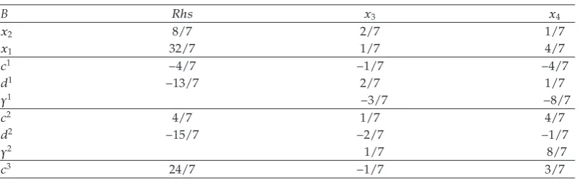
Table1
B Rhs x3 x4
x2 8/7 2/7 1/7
x1 32/7 1/7 4/7
c1 −4/7 −1/7 −4/7
d1 −13/7 2/7 1/7
γ1 −3/7 −8/7
c2 4/7 1/7 4/7
d2 −15/7 −2/7 −1/7
γ2 1/7 8/7
c3 24/7 −1/7 3/7
4. An illustrative example
The following program P is given as an example of multiple objective linear fractional programmingMOLFPin Kornbluth and Steuer20:
maxZ1x x1−4
−x2 3,
maxZ2x −x1 4 x2 1 ,
maxZ3x −x1 x2, subject to−x1 4x2≤0,2x1−x2≤8, x1≥0, x2≥0,and integers.
4.1
Using the described algorithm, programP0is first resolved and the optimal solution is given in the simplexTable 1:
Sinceγj1 ≤ 0 for allj ∈ J01,J01 N0 {3,4}, then the obtained solution32/7,8/7is optimal for programP0, but not integer. Therefore, two branches are possible.
1x1≥5⇔ −1/7x3−4/7x4≥3/7. This is not possible and1is fathomed.
2x1≤4⇔ −1/7x3−4/7x4≤ −4/7.
This constraint is added and the dual simplex method is applied. The integer optimal solution of programP2is obtained inTable 2.
γ1
j ≤ 0 for allj ∈J21,J21 N2 {3,5}, then the current solution4,1is optimal. Eff :
{4,1},H2{5},andS3{x∈S2|x5≥1}.
The constraintx5≥1 is added to the current simplex table and after pivoting, we obtain
Table 3.
J1
3 ∅then,3,0is an optimal integer solution and Eff :{4,1,3,0}.
Proceeding in this manner, we obtainTable 4.
J1
4 ∅then,0,0is an optimal integer solution, Eff :{4,1,3,0,0,0},N4{1,10}, H4{10},andS5{x∈S4|x10≥1}.
The constraintx10≥1 is added and we obtainTable 5.
The dual is not feasible, then the corresponding node is fathomed.
[image:9.600.98.506.109.236.2]Table2
B Rhs x3 x5
x2 1 1/4 1/4
x1 4 0 1
x4 1 1/4 −7/4
c1 0 0 −1
d1 −2 1/4 1/4
γ1 0 −2
c2 0 0 1
d2 −2 −1/4 −1/4
γ2 0 2
c3 3 −1/4 3/4
Table3
B Rhs x2 x6
x3 3 4 1
x1 3 0 1
x4 2 −1 −2
x5 1 0 −1
c1 1 0 −1
d1 −3 −1 0
γ1 −1 −3
c2 −1 0 1
d2 −1 1 0
γ2 −1 1
c3 3 1 1
Table4
B Rhs x1 x10
x6 3 1 0
x3 0 1 4/3
x4 8 1 −1
x5 4 1 0
x7 2 0 −1
x9 1 3 8
x8 0 1 1
x2 0 −1 −1
c1 4 1 0
d1 −3 −1 −1
γ1 −1 −4
c2 −4 −1 0
d2 −1 1 1
γ2 −5 −4
Table5
Rhs x11 x10
x6 2 1 −1
x3 −1 1 1/3
x4 7 1 −2
x5 3 1 −1
x7 2 0 −1
x9 −2 3 5
x8 −1 1 0
x2 1 −1 0
x1 1 −1 1
c1 3 1 −1
d1 −2 −1 0
γ1 −1 −4
c2 −3 −1 1
d2 −2 1 0
γ2 −5 −4
c3 0 0 1
Table6
n, m, α, 15,10,33 20,10,25 25,5,17 25,10,17
Efficient Mean 99,50 204,50 200,45 98,00
Solutions Max 215 324 397 228
Min 4 23 67 17
CPU Mean 38,52 185,96 400,48 306,74
second Max 54,39 337,08 673,17 367,11
Min 23,094 143,56 193,87 177,09
Simplex Mean 75837,7 126488,50 521763,45 255726,55
Iterations Max 101207 365750 719105 306665
Min 55851 2717 369414 145324
Efficient Mean 885,3 2341,50 2607,15 979,00
CutsEC Max 1152 2593 3909 1268
Min 451 679 839 440
EC/Cuts Mean 0,91 0,97 0,84 0,81
5. Computational results
The computer program was coded in MATLAB 7.0 and run on a 3.40 GHz DELL pentium 4, 1.00 GB RAM. The used software was developed by the authors and was tested on randomly generated problems. We show the results of the computational experiment inTable 6.
integer values of the matrix constraints vary in the interval1,50and for those of criteria in
1,30.The right-hand side value is set to α% of the sum of the coefficientsinteger partof each constraint, whereα∈ {17,25,33}. With each instancen, m, α,a series of 20 problems is solved and the whole efficient solution set was generated for all these problems.
The method being exact, it was expected that the iteration number of the simplex method is very large taking into account the fact that, for this type of problems, the number of efficient solutions increases quickly with the data size. In addition, we should like to point out that the ratio EC/cuts tends toward the value one, showing that the number of efficient cuts introduced into the method is very large compared to the full number of cuts and indicating that this type of cuts has a positive impact on the research of the whole of efficient solutions.
6. Conclusion
In this paper, an exact method for generating all efficient solutions for multiple objective integer linear fractional programming problems is presented The method does not require any nonlinear optimization. A linear fractional program is solved using the Cambini and Martein’s algorithm in the original format and then by using the well-known concept of branching in integer linear programming, integer solutions are generated. The proposed efficient cut exploits all the criteria in the simplex table, and only the parts of the feasible solutions domain containing efficient solutions are explored. Also it is easy to implement the proposed cut since to obtain integer solutionxk 1 from xk,one has just to append the cut in the simplex
table corresponding toxkand carry out pivoting iterations as in an ordinary linear fractional
programming problem. The described method solves MOILFP problems in the general case. However, in order to make the algorithm more powerful, the tree structure of the algorithm can be exploited for construction of a parallel algorithm. For large scale problems, the number of efficient solutions can be very high so that it becomes unrealistic to generate them all. In this case, one can choose only the increasing directions of criteria which satisfy a desirable augmentation. This can be made by building the setsHlin an interactive way at each step of
the algorithm.
Acknowledgments
The authors are grateful to anonymous referees for their substantive comments that improved the content and presentation of the paper. This research has been completely supported by the laboratory LAID3 of the High Education Algerian Ministry.
References
1 S. Schaible, “Fractional programming: applications and algorithms,”European Journal of Operational Research, vol. 7, no. 2, pp. 111–120, 1981.
2 A. Nagih and G. Plateau, “Probl`emes fractionnaires: tour d’horizon sur les applications et m´ethodes de r´esolution,”RAIRO Operations Research, vol. 33, no. 4, pp. 383–419, 1999.
3 B. D. Craven,Fractional Programming, vol. 4 ofSigma Series in Applied Mathematics, Heldermann, Berlin, Germany, 1988.
4 I. M. Stancu-Minasian,Fractional Programming: Theory, Methods and Applications, vol. 409 ofMathematics and Its Applications, Kluwer Academic Publishers, Dordrecht, The Netherlands, 1997.
6 J. B. G. Frenk and S. Schaible, “Fractional programming: Introduction and Applications,” in
Encyclopedia of Optimization, C. A. Floudas and P. M. Pardalos, Eds., pp. 162–172, Kluwer Academic Publishers, Dordrecht, The Netherlands, 2001.
7 I. M. Stancu-Minasian, “A sixth bibliography of fractional programming,”Optimization, vol. 55, no. 4, pp. 405–428, 2006.
8 I. M. Stancu-Minasian, “A fifth bibliography of fractional programming,”Optimization, vol. 45, no. 1– 4, pp. 343–367, 1999.
9 R. E. Steuer, Multiple Criteria Optimization: Theory, Computation, and Application, Wiley Series in Probability and Mathematical Statistics: Applied Probability and Statistics, John Wiley & Sons, New York, NY, USA, 1986.
10 A. Cambini and L. Martein, “Equivalence in linear fractional programming,”Optimization, vol. 23, no. 1, pp. 41–51, 1992.
11 A. Charnes and W. W. Cooper, “Programming with linear fractional functionals,” Naval Research Logistics Quarterly, vol. 9, no. 3-4, pp. 181–186, 1962.
12 D. Granot and F. Granot, “On integer and mixed integer fractional programming problems,” in
Studies in Integer Programming, vol. 1 ofAnnals of Discrete Mathematics, pp. 221–231, North-Holland, Amsterdam, The Netherlands, 1977.
13 B. Martos,Nonlinear Programming: Theory and Method, North-Holland, Amsterdam, The Netherlands, 1975.
14 C. R. Seshan and V. G. Tikekar, “Algorithms for integer fractional programming,”Journal of the Indian Institute of Science, vol. 62, no. 2, pp. 9–16, 1980.
15 M. Abbas and M. Moula¨ı, “Integer linear fractional programming with multiple objective,”Journal of the Italian Operations Research Society, vol. 32, no. 103-104, pp. 15–38, 2002.
16 R. Caballero and M. Hern´andez, “The controlled estimation method in the multiobjective linear fractional problem,”Computers & Operations Research, vol. 31, no. 11, pp. 1821–1832, 2004.
17 A. Cambini, L. Martein, and I. M. Stancu-Minasian, “A survey of bicriteria fractional problems,”
Advanced Modeling and Optimization, vol. 1, no. 1, pp. 9–46, 1999.
18 M. Chakraborty and S. Gupta, “Fuzzy mathematical programming for multi objective linear fractional programming problem,”Fuzzy Sets and Systems, vol. 125, no. 3, pp. 335–342, 2002.
19 J. P. Costa, “Computing non-dominated solutions in MOLFP,”European Journal of Operational Research, vol. 181, no. 3, pp. 1464–1475, 2007.
20 J. S. H. Kornbluth and R. E. Steuer, “Multiple objective linear fractional programming,”Management Science, vol. 27, no. 9, pp. 1024–1039, 1981.
21 B. Metev and D. Gueorguieva, “A simple method for obtaining weakly efficient points in multiobjective linear fractional programming problems,” European Journal of Operational Research, vol. 126, no. 2, pp. 386–390, 2000.
22 O. M. Saad and J. B. Hughes, “Bicriterion integer linear fractional programs with parameters in the objective functions,”Journal of Information & Optimization Sciences, vol. 19, no. 1, pp. 97–108, 1998.
23 M. Ehrgott and X. Gandibleux, “An annotated bibliography of multiobjective combinatorial optimization,” Report in Wissenschaftmathematik no. 62, Fachbereich Mathematik, Universitat Kaiserslautern, Kaiserslautern, Germany, 2000.