Munich Personal RePEc Archive
A Generalized Quality-Ladder Growth
Model with Patent Breadth: Quantifying
the Effects of Blocking Patents on RD
Chu, Angus C.
University of Michigan
August 2007
Online at
https://mpra.ub.uni-muenchen.de/4746/
A Generalized Quality-Ladder Growth Model with Patent Breadth: Quantifying the Effects of Blocking Patents on R&D
Angus C. Chu* University of Michigan
August 2007
Abstract
Why is there so little R&D in the US? To quantify the effects of blocking patents on R&D, this
paper firstly develops a tractable framework to model the transition dynamics of an economy with patent
breadth and blocking patents in a generalized quality-ladder growth model. In this dynamic
general-equilibrium setting, a dynamic distortion on capital accumulation that has been neglected by previous
studies on patent policy is identified. Then, the model is applied to the aggregate data to quantify the
extents of underinvestment in R&D and inefficiency arising from blocking patents. This numerical
exercise suggests a number of findings. Firstly, the market economy underinvests in R&D so long as a
non-negligible fraction of long-run TFP growth is driven by R&D. Secondly, eliminating blocking patents
increases R&D by about two to six times and hence is an effective solution to the potential problem of
R&D underinvestment. Finally, the effects of eliminating blocking patents on consumption in the long
run and during the transition dynamics are considered.
Keywords: blocking patents, endogenous growth, intellectual property rights, patent breadth, R&D
JEL classification: O31, O34
*
“Today, most basic and applied researchers are effectively standing on top of a huge
pyramid… Of course, a pyramid can rise to far greater heights than could any one
person... But what happens if, in order to scale the pyramid and place a new block on the
top, a researcher must gain the permission of each person who previously placed a block
in the pyramid, perhaps paying a royalty or tax to gain such permission? Would this
system of intellectual property rights slow down the construction of the pyramid or limits
its heights? … To complete the analogy, blocking patents play the role of the pyramid’s
building blocks.” – Carl Shapiro (2001)
1. Introduction
What are the effects of blocking patents on research and development (R&D)? In an environment with
only horizontal innovations, each invention is a different variety from each other. In this setting, a higher
level of patent breadth increases the differentiability of each product that potentially results in a higher
markup, a larger amount of monopolistic profits, and consequently, enhanced incentives for R&D. In a
more complicated and realistic environment with sequential innovations, patent breadth takes the form of
lagging breadth and leading breadth. Lagging breadth provides patent protection against imitation while
leading breadth provides patent protection against subsequent innovations, which may infringe existing
patents. A broadening of leading breadth may enhance or dampen the incentives for R&D depending on
the extent of blocking patents, which is determined by the profit-sharing rule in patent pools.
To quantify the effects of blocking patents on R&D and consumption, this paper firstly develops
a tractable framework to model the transition dynamics of an economy with patent breadth and blocking
patents in a generalized quality-ladder growth model. In this dynamic general-equilibrium (DGE) setting,
this paper analytically derives and identifies a dynamic distortionary effect on capital accumulation, which has been neglected by previous studies on patent policy focusing mostly on the static distortionary
effect of markup pricing. Then, the model is applied to the aggregate data of the US’s economy in order
The numerical exercise suggests a number of findings. Firstly, eliminating blocking patents
increases the equilibrium amount of R&D spending by about two to six times. Secondly, the market
economy underinvests in R&D relative to the first-best optimum so long as a non-negligible fraction of
long-run total factor productivity (TFP) growth is driven by R&D. To understand this finding, the
quality-ladder growth model involves multiple externalities in R&D: (a) a negative intratemporal congestion or
duplication externality; (b) a positive or negative externality in intertemporal knowledge spillover; (c) the
static consumer-surplus appropriability problem which is a positive externality; (d) the dynamic surplus
appropriability problem in the form of sequential innovations which is a also a positive externality; (e) the
business-stealing effect from creative destruction which is a negative externality; and (f) the negative
effects of blocking patents on R&D in the case of suboptimal profit-sharing rules in patent pools. Given
the existence of positive and negative externalities, whether the market economy over or under-invests in
R&D depends crucially on the extents of intratemporal duplication and intertemporal spillover, which in
turn are imputed from the balanced-growth condition between long-run TFP growth and R&D. Therefore,
the larger is the fraction of long-run TFP growth driven by R&D, the more likely it is for the market
economy to underinvest in R&D. Finally, the effects of eliminating blocking patents on consumption in
the long run and during the transition dynamics are considered. When blocking patents are eliminated, the
balanced-growth level of consumption increases significantly so long as a non-negligible fraction of TFP
is driven by R&D. During the transition dynamics, the economy does not always experience a significant
fall in consumption in response to the resource reallocation away from the production sector to the R&D
sector. Over a range of parameters, upon eliminating blocking patents, consumption gradually rises
towards the new balanced-growth path by reducing physical investment and temporarily running down
the capital stock. This finding contrasts with Kwan and Lai (2003), whose model does not feature capital
accumulation and hence predicts consumption losses from resource reallocation during the transition path.
Shapiro (2001) describes the current innovation process as a “dense web of overlapping
intellectual property rights that a company must hack its way through in order to actually commercialize
framework to evaluate the effects of this patent thicket on R&D and provides an effective solution to the
potential problem of R&D underinvestment identified by Jones and Williams (1998) and (2000). Jones
and Williams (1998) develop a method to calculate the social rate of return to R&D based on
endogenous-growth theory and find that the socially optimal amount of R&D spending is at least two to
four times larger than the actual amount. Jones and Williams (2000) adopt a different approach by
calibrating a variety-expanding growth model to the data and obtain a similar conclusion that there is
underinvestment in R&D over a wide range of parameters.1 The current paper follows this latter approach
by calibrating a generalized quality-ladder growth model with patent breadth in sequential innovations to
show that the potential problem of R&D underinvestment arises from the inefficiency of blocking patents
and eliminating them can be an effective solution. Furthermore, the calibration exercise takes into
consideration Comin’s (2004) critique that long-run TFP growth may not be solely driven by R&D.
The current paper also complements the theoretical and qualitative studies on leading breadth
from the patent-design literature,2 such as Green and Scotchmer (1995), O’Donoghue et al (1998) and Hopenhayn et al (2006), by providing a quantitative DGE analysis using the aggregate data. O’Donoghue
and Zweimuller (2004) is the first study that merges the patent-design and endogenous growth literatures
to analyze the effects of patentability requirement, lagging and leading breadth on economic growth in a
simple quality-ladder growth model. However, their focus was not in quantifying the effects of blocking
patents on R&D. In addition, the current paper generalizes their model in a number of dimensions in order
to perform a quantitative analysis on the transition dynamics. Goh and Olivier (2002) analyze the welfare
effects of patent breadth in a two-sector variety-expanding growth model, and Grossman and Lai (2004)
analyze the welfare effects of strengthening patent protection in developing countries as a result of the
TRIPS agreement using a multi-country variety-expanding model. However, these studies do not analyze
patent breadth in an environment with sequential innovations. Li (2001) analyzes the optimal policy mix
1
Stokey (1995) also calibrates an R&D-growth model to examine the extents of R&D underinvestment in the market economy.
2
of R&D subsidy and lagging breadth in a quality-ladder model with endogenous step size, but he does not
consider leading breadth. Furthermore, all the abovementioned studies are qualitatively oriented and do
not feature capital accumulation so that the dynamic distortion is absent.
Laitner (1982) identifies in an exogenous growth model with overlapping generations of
households that the existence of an oligopolistic sector and its resulting pure profits as financial assets
creates both the usual static distortion and an additional dynamic distortion on capital accumulation due to
the crowding out of households’ portfolio space, and he finds that the latter is more significant than the
former. The current paper extends this study to show that this dynamic distortion also plays an important
role and through a different channel in an R&D-driven endogenous growth model in which both patents
and physical capital are owned by households as financial assets.
In terms of quantitative analysis, this paper relates to Kwan and Lai (2003) and Chu (2007).
Kwan and Lai (2003) numerically evaluate the effects of extending the effective lifetime of patent in the
variety-expanding model originating from Romer (1990) and find substantial welfare gains despite the
temporary consumption losses during the transition path in their model. Chu (2007) uses a generalized
variety-expanding model and finds that whether or not an extension in the patent length is effective in
stimulating R&D depends crucially on the patent-value depreciation rate. At the empirical range of
patent-value depreciation rates estimated by previous studies, patent extension has only limited effects on
R&D and thus social welfare. Therefore, Chu (2007) and the current paper together provide a comparison
on the effectiveness of increasing patent length and eliminating blocking patents in solving the R&D
underinvestment problem. The crucial difference between these two policy instruments arises because
patent extension increases future monopolistic profits while eliminating blocking patents raises current
monopolistic profits for the inventors.
The rest of the paper is organized as follows. Section 2 describes the model. Section 3 calibrates
the model and numerically evaluates the effects of eliminating blocking patents. The final section
2. The Model
The model is a generalized version of Grossman and Helpman (1991) and Aghion and Howitt (1992). To
prevent the model from overestimating the social benefits of R&D and hence the extents of R&D
underinvestment, long-run TFP growth is assumed to be driven by R&D as well as an exogenous process
as in Comin (2004). In order to perform a more realistic calibration, the model is further modified to
include physical capital, which is a factor input for the production of intermediate goods and R&D, and
the final goods can be used for consumption or investment in capital. Finally, the class of first-generation
R&D-driven endogenous growth models, such as Grossman and Helpman (1991) and Aghion and Howitt
(1992), exhibits scale effects and is inconsistent with the empirical evidence in Jones (1995a).3 In the
present model, scale effects are eliminated by assuming decreasing individual R&D productivity as in Segerstrom (1998), which becomes a semi-endogenous growth model.4
The various components of the model are presented in Sections 2.1–2.7, and the decentralized
equilibrium is defined in Section 2.8. Section 2.9 summarizes the laws of motion that characterize the
transition dynamics, and Section 2.10 analyzes the balanced-growth path. Section 2.11 derives the
first-best optimal allocations.
2.1. Representative Household
The infinitely-lived representative household maximizes life-time utility that is a function of per-capita
consumption
c
t of the numeraire final goods and is assumed to have the iso-elastic form given by(1)
U
e
ntc
tdt
σ
σ ρ
−
=
− ∞
− −
1
1
0 ) (
.
3
See, e.g. Jones (1999) for an excellent theoretical analysis on scale effects.
4
1
≥
σ
is the inverse of the elasticity of intertemporal substitution. The household hasL
t=
L
0exp(n
.t
)members at time t. The population size at time 0 is normalized to one, and n>0 is the exogenous population growth rate.
ρ
is the subjective discount rate. To ensure that lifetime utility is bounded, it isassumed that
ρ
>n. The household maximizes (1) subject to a sequence of budget constraints given by(2) at =at(rt −n)+wt −ct.
Each member of the household inelastically supplies one unit of homogenous labor in each period to earn
a real wage income wt. at is the value of risk-free financial assets in the form of patents and physical
capital owned by each household member, and rt is the real rate of return on these assets. The familiar
Euler equation derived from the intertemporal optimization is
(3) ct =ct(rt −
ρ
)/σ
.2.2. Final Goods
This sector is characterized by perfect competition, and the producers take both the output price and input
prices as given. The production function for the final goods Yt is a Cobb-Douglas aggregator of a
continuum of differentiated quality-enhancing intermediate goods Xt(j) for j∈[0,1] given by
(4) =
1
0
) ( ln
exp X j dj
Yt t .
5
The familiar aggregate price index is
(5) exp ln ( ) 1
1
0
=
= P j dj
Pt t ,
5
and the demand curve for each variety of intermediate goods is
(6) Pt(j)Xt(j)=Yt.
2.3. Intermediate Goods
There is a continuum of industries producing the differentiated quality-enhancing intermediate goods
) (j
Xt for j∈[0,1]. A fraction
θ
∈[0,1) of the industries is characterized by perfect competitionbecause innovations in these industries are assumed to be non-patentable. Each of the remaining
industries is dominated by a temporary industry leader, who owns the patent for the latest R&D-driven
technology for production. Without loss of generality, the industries are ordered such that industries
) , 0
[
θ
∈ ′
j are competitive and industries j∈[θ,1] are monopolistic. The production function in each
industry has constant returns to scale in labor and capital inputs and is given by
(7)
X
(
j
)
z
( )Z
tK
x,t(
j
)
L
1x,t(
j
)
jm t
t α −α
=
for j∈[0,1]. Kx,t(j) and Lx,t(j) are respectively the capital and labor inputs for producing
intermediate-goods j at time t. Zt =Z0exp(gZt) represents an exogenous process of productivity
improvement that is common across all industries and is freely available to all producers. zmt(j) is
industry j’s level of R&D-driven technology, which is increasing over time through R&D investment and
successful innovations. z>1 is the exogenous step-size of a technological improvement arising from
each innovation. mt(j), which is an integer, is the number of innovations that has occurred in industry j
as of time t. The marginal cost of production in industry j is
(8)
α α
α
α
−
−
=
1 )
(
1
1
)
(
t tt j m t
w
R
Z
z
j
MC
t ,
where Rt is the rental price of capital. The optimal price for the leaders in the monopolistic industries is a
(9) Pt(j)=
µ
(z,η
)MCt(j)for j∈[θ,1]. The markup
µ
(z,η
) is a function of the quality step size z and the level of patent breadthη
(to be defined in Section 2.4). The competitive industries are characterized by competitive pricing suchthat
(10) Pt(j′)=MCt(j′)
for j′∈[0,
θ
). The aggregate price level is(11) Pt =
µ
~(z,η
,θ
)MCt,where
µ
~(z,η
,θ
)≡µ
(z,η
)1−θ is the aggregate markup in the economy. The aggregate marginal cost is(12) =
1
0
) ( ln
exp MC j dj
MCt t .
2.4. Patent Breadth
Before providing the underlying derivations, this section firstly presents the Bertrand equilibrium price
and the amount of monopolistic profits generated by an invention and captured by a patent pool under
different levels of patent breadth, which is denoted by
η
.(13) Pt(j)=zηMCt(j)
(14)
π
t(j)=(zη −1)MCt(j)Xt(j)for
η
∈{1,2,3,...} and j∈[θ,1]. The expression for the equilibrium price is consistent with the seminalwork of Gilbert and Shapiro’s (1990) interpretation of “breadth as the ability of the patentee to raise
price.” A broader patent breadth corresponds to a larger
η
, and vice versa. Therefore, an increase inpatent breadth potentially enhances the incentives for R&D by raising the amount of monopolistic profits
The patent-design literature has identified and analyzed two types of patent breadth in an
environment with sequential innovations: (a) lagging breadth; and (b) leading breadth. In a standard
quality-ladder growth model, lagging breadth (i.e. patent protection against imitation) is assumed to be
complete while leading breadth (i.e. patent protection against subsequent innovations) is assumed to be
zero. The following analysis focuses on non-zero leading breadth, and the formulation originates from
O’Donoghue and Zweimuller (2004). A discussion of incomplete lagging breadth is in Appendix II.
The level of patent breadth
η
=η
lag +η
lead can be decomposed into lagging breadth denoted by] 1 , 0 (
∈
lag
η
and leading breadth denoted byη
lead ∈{0,1,2,...}. In the following, complete laggingbreadth is assumed such that
η
=1+η
lead. Nonzero leading breadth protects patentholders againstsubsequent innovations and gives the patentholders property rights over future inventions. For example, if
1
=
lead
η
, then the most recent innovation infringes the patent of the second-most recent inventor. If2
=
lead
η
, then the most recent innovation infringes the patents of the second-most and the third-mostrecent inventors, etc. The following diagram illustrates the concept of nonzero leading breadth with an
example of leading breadth equal two.
Therefore, nonzero leading breadth facilitates the new industry leader and the previous inventors, whose
patents are infringed, to consolidate market power through licensing agreements and the formation of a
patent pool resulting in a higher markup.6 The Bertrand equilibrium price with leading breadth is
(15) Pt(j)=z1+ηleadMCt(j)
for
η
lead ∈{0,1,2,...} and j∈[θ,1]. Assumption 1 is sufficient to derive this equilibrium markup price.6
See, e.g. Gallini (2002) and O’Donoghue and Zweimuller (2004), for a discussion on market-power consolidation through licensing agreements.
) (j mt
z zmt(j)+2
patent protection for zmt(j)
1 ) (j+
mt
Assumption 1: An infringed patentholder cannot become the next industry leader while she is still covered by a licensing agreement in that industry.7
Then, the total amount of monopolistic profits captured by the patent pool at time t is
(16)
π
t(j)=(z1+ηlead −1)MCt(j)Xt(j)for
η
lead ∈{0,1,2,...} and j∈[θ,1].The share of profits obtained by each generation of patentholders in the patent pool depends on
the profit-sharing rule (i.e. the terms in the licensing agreement). A stationary bargaining outcome is
assumed to simplify the analysis.
Assumption 2: The set of profit-sharing rule is symmetric across industries and is stationary. For each degree of leading breadth ηlead ∈{0,1,2,...}, the profit-sharing rule is σηlead =(σ1,...,ση)∈[0,1], where
i
σ is the share of profits received by the i-th most recent inventor, and =1 =1
η σ
i i .
Although the shares of profits and licensing fees eventually received by the owner of an invention are
constant overtime, the present value of profits is determined by the actual profit-sharing rule. The two
extreme cases are: (a) complete frontloading
σ
ηlead =(1,0,...,0); and (b) complete backloading) 1 ,..., 0 , 0 (
= lead
η
σ
. Complete frontloading maximizes the incentives on R&D provided by leadingbreadth by maximizing the present value of profits received by an inventor. The opposite effect of
blocking patents arises when profits are backloaded, and complete backloading maximizes this damaging
7
effect on the incentives for R&D. Section 2.7 derives the law of motion for the market value of ownership
in patent pools for each generation of patentholders.
2.5. Aggregation
Define At ≡exp mt(j)djlnz
1
0
as the aggregate level of R&D-driven technology. Also, define total
labor and capital inputs for production as
=
1
0 ,
,
K
(
j
)
dj
K
xt xt and=
1
0 ,
,
L
(
j
)
dj
L
xt xt respectively.Lemma 1: The aggregate production function for the final goods is (17)
Y
t=
ϑ
(
η
)
A
tZ
tK
xα,tL
1x−,tα,where
ϑ
(η
)≡( η)θ /( ηθ
+1−θ
)z
z is decreasing in
η
forθ
∈(0,1).) (
η
ϑ
represents the static distortionary effect of markup pricing. Markup pricing in the monopolisticindustries distorts production towards the competitive industries and reduces the output of the final goods.
Also,
ϑ
(η) is initially decreasing inθ
and subsequently increasing withϑ
(η
)=1 forθ
∈{0,1}.Therefore, at least over a range of parameters, the static distortionary effect becomes increasingly severe
as the fraction of competitive industries increases.
The market-clearing condition for the final goods is
(18) Yt =Ct +It,
where Ct =Ltct is the aggregate consumption and It is the investment in physical capital. The factor
payments for the final goods are
=
1)
(
θ
π
π
t tj
dj
is the total amount of monopolistic profits. Substituting (7) and (8) into (14) and thensumming over all monopolistic industries yields
(20) t
Y
tz
z
−
−
=
ηη
θ
π
(
1
)
1
.Therefore, the growth rate of monopolistic profits equals the growth rate of output. The amount of factor
payments for labor and capital inputs in the intermediate-goods sector are respectively
(21) t xt
Y
tz
z
L
w
=
−
+
η−
η
θ
θ
α
)
1
1
(
, ,
(22) t xt
Y
tz
z
K
R
=
+
η−
η
θ
θ
α
1
, .
(22) shows that the markup drives a wedge between the marginal product of capital and its rental price.
As will be shown below, this wedge creates a distortion on the rate of investment in physical capital.
Finally, the correct value of gross domestic product (GDP) should include the amount of investment in
R&D such that
(23) GDPt =Yt +wtLr,t +RtKr,t.8
t r
L, and Kr,t are respectively the number of workers and the amount of capital for R&D.
2.6. Capital Accumulation
The market-clearing condition for physical capital is
(24) Kt =Kx,t +Kr,t.
t
K is the total amount of capital available in the economy at time t. The law of motion for capital is
8
(25) Kt = It −Kt
δ
δ
is the rate of depreciation. The endogenous rate of investment in physical capital is(26) it =(Kt/Kt +
δ
)Kt/Ytfor all t. The no-arbitrage condition rt =Rt −
δ
for the holding of capital and (22) imply that thecapital-output ratio is
(27)
) )( 1
(
) 1 (
,
δ
θ
θ
α
ηη
+ −
− + =
t t K t
t
r s z
z Y
K
.
t K
s , is the endogenous share of capital in the R&D sector. Substituting (27) into (26) yields
(28)
+
+
−
−
+
=
δ
δ
θ
θ
α
η η
t t t t
K t
r
K
K
s
z
z
i
/
)
1
(
)
1
(
,
.
In the Romer model, (skilled) labor is the only factor input for R&D (i.e. sK,t =0); therefore, the
distortionary effect of markup pricing on the steady-state rate of investment is unambiguously negative
(i.e. ∂i/∂
η
<0). In the current model, there is an opposing positive effect operating through the R&Dshare of capital. Intuitively, an increase in patent breadth potentially raises the private return on R&D and
increases the R&D share of capital. Proposition 2 in Section 2.11 shows that the negative distortionary
effect still dominates if the intermediate-goods sector is at least as capital intensive as the R&D sector.
2.7. R&D
) (j
Vt is the market value of the patent pool created by the most recent invention in industry j∈[θ,1] at
time t and is determined by the following no-arbitrage condition
(29) rtVt(j)=
π
t(j)+Vt(j)−λ
tVt(j).The first terms in the right is the flow profits generated by the patent pool at time t. The second term is the
capital gain due to the growth in the amount of monopolistic profits. The third term is the expected value
creates a new patent pool. However, the incentives for R&D depend on the market value of the shares in
patent pools obtained by an inventor. Denote Vi,t(j) for i∈{1,...,
η
} as the market value of ownership inpatent pools for the i-th most recent inventor in industry j∈[θ,1].
Proposition 1:Vi,t(j) for i∈{1,2,...,
η
} and j∈[θ,1] is determined by the following law of motion(30)
r
tV
i,t(
j
)
=
σ
iπ
t(
j
)
+
V
i,t(
j
)
+
λ
t(
V
i+1,t(
j
)
−
V
i,t(
j
))
,where Vη+1,t(j)=0. The no-arbitrage condition for V1,t(j) can be re-expressed as
(31)
− +
=
∏
= = −
η
λ
λ
σ
π
1 1 , ,
1 ,
1
) ( / ) ( 1 )
( ) (
k
k
i t t it it k
t k t
t
j V j V r
j j
V .
Assumption 4: Innovation successes of the R&D entrepreneurs are randomly assigned to the industries in the intermediate-goods sector.
The expected present value of an invention obtained by the most recent inventor at time t is
(32)
− + −
− =
=
∏
= = −
η
η η
θ
λ
λ
σ
θ
1 1 , ,
1 1
, 1 , 1
/ 1 1
) 1 ( ) (
k
k
i t t it it k
t k t t
t
V V r
Y z z dj
j V
V .
The arrival rate of an innovation success for an R&D entrepreneur h∈[0,1] is a function of labor input
) (
, h
Lrt and capital input Kr,t(h) given by
(33) t
(
h
)
tK
r,t(
h
)
L
1r,t(
h
)
β β
ϕ
λ
−=
.9t
ϕ
is a productivity parameter that the entrepreneurs take as given. The expected profit from R&D is(34) Et[
π
r,t(h)]=V1,tλ
t(h)−wtLr,t(h)−RtKr,t(h).9
The first-order conditions are
(35)
(
1
−
β
)
V
1,tϕ
t(
K
r,t(
h
)
/
L
r,t(
h
))
β=
w
t,(36)
V
t tK
rth
L
rth
−1=
R
t, ,
,
1
(
(
)
/
(
))
β
ϕ
β
.To eliminate scale effects and capture various externalities, the individual R&D productivity parameter
ϕ
t at time t is assumed to be decreasing in the level of R&D-driven technology At such that(37) φ
γ β β
ϕ
ϕ
−− −
= 1
1 1
,
, )
(
t t r t r t
A L K
,
where
=
1
0 ,
,
K
(
h
)
dh
K
rt rt and=
1
0 ,
,
L
(
h
)
dh
L
rt rt .γ
∈(0,1] captures the intratemporal negativecongestion or duplication externality or the so-called “stepping on toes” effects, and
φ
∈(−∞,1) capturesthe externality of intertemporal knowledge spillovers.10 Given that the arrival of innovations follows a
Poisson process, the law of motion for R&D-driven technology is given by
(38)
A
tA
tλ
tln
z
A
tϕ
tK
rβ,tL
1r−,tβln
z
A
tφ(
K
rβ,tL
1r−,tβ)
γϕ
ln
z
=
=
=
.112.8. Decentralized Equilibrium
The analysis starts at t=0. The equilibrium is a sequence of prices
{
w
t,
r
t,
R
t,
P
t(
j
),
V
1,t}
t∞=0 and asequence of allocations
{
a
t,
c
t,
I
t,
Y
t,
X
t(
j
),
K
x,t(
j
),
L
x,t(
j
),
K
r,t(
h
),
L
r,t(
h
),
K
t,
L
t}
∞t=0 such that they are10
This specification captures how semi-endogenous growth models eliminate scale effects as in Jones (1995b). )
1 , 0 (
∈
φ corresponds to the “standing on shoulder” effect, in which the economy-wide R&D productivity Aqϕ
increases as the level of R&D-driven technology increases (see the law of motion for R&D-driven technology). On the other hand, φ∈(−∞,0) corresponds to the “fishing out” effect, in which early technology is relatively easy to develop and Aqϕ decreases as the level of R&D-driven technology increases.
11
This convenient expression is derived as A m j dj z d z
t
t
t ( ) ln ( ) ln
ln
0 1
0
=
= λ τ τ ; then, simple differentiation
consistent with the initial conditions {K0,L0,Z0,A0,
ϕ
0} and their subsequent laws of motions. Also, ineach period,
(a) the representative household chooses {at,ct} to maximize utility taking {wt,rt} as given;
(b) the competitive firms in the final-goods sector choose {Xt(j)} to maximize profits according to
the production function taking {Pt(j)} as given;
(c) each industry leader in the intermediate-goods sector chooses {Pt(j),Kx,t(j),Lx,t(j)} to
maximize profits according to the Bertrand price competition and the production function taking
} ,
{Rt wt as given;
(d) the competitive firms in the intermediate-goods sector choose {Kx,t(j′),Lx,t(j′)} to maximize
profits according to the production function taking {Pt(j′),Rt,wt} as given;
(e) each entrepreneur in the R&D sector chooses {Kr,t(h),Lr,t(h)} to maximize profits according to
the R&D production function taking {
ϕ
t,V1,t,Rt,wt} as given;(f) the market for the final-goods clears such that Yt =Ct +It;
(g) the full employment of capital such that Kt =Kx,t +Kr,t; and
(h) the full employment of labors such that Lt = Lx,t +Lr,t.
2.9. Transition Dynamics
The transition dynamics of the decentralized equilibrium is characterized by the following differential
equations. The capital stock is a predetermined variable and evolves according to
(39) Kt =Yt −Ct−Kt
δ
.R&D-driven technology is also a predetermined variable and evolves according to
Consumption is a jump variable and evolves according to the Euler equation
(41) ct =ct(rt −
ρ
)/σ
.The market value of ownership in patent pools is also a jump variable and evolves according to
(42)
V
i,t=
(
r
t+
λ
t)
V
i,t−
λ
tV
i+1,t−
σ
iπ
tfor i∈{1,2,...,
η
} and Vη+1,t =0.At the aggregate level, the generalized quality-ladder model is similar to Jones’s (1995b) model,
whose dynamic properties have been investigated by a number of recent studies. For example, Arnold
(2006) analytically derives the uniqueness and local stability of the steady state with certain parameter
restrictions. Steger (2005) and Trimborn et al (2006) numerically evaluate the transition dynamics of the
model. In summary, to solve the model numerically, I firstly transform {Kt,At,ct,Vi,t} in the differential
equations into its stationary form,12 and then, compute the transition path from the old steady state to the
new one using the relaxation algorithm developed by Trimborn et al (2006).
2.10. Balanced-Growth Path
Equating the first-order conditions (21) and (35) and imposing the balanced-growth condition on
R&D-driven technology
(43)
g
A tL
rtK
r,tln
z
1 ,
β β
ϕ
−=
yield the steady-state R&D share of labor inputs given by
(44)
(
)
)
1
(
)
1
)(
1
(
1
1
1
lead
z
z
g
r
s
s
Y L
L η
η η
σ
ν
θ
θ
θ
λ
λ
α
β
−
+
−
−
−
+
−
−
=
−
,12
where ( ) (0,1] 1 1 ∈ − + ≡ = − η η
λ
λ
σ
σ
ν
k k Y k g rlead is defined as the backloading discount factor. For
example, in the case of complete frontloading,
ν
(σ
ηlead)=1. Similarly, solving (22), (36) and (43) yieldsthe steady-state R&D share of capital inputs given by
(45)
(
)
)
1
(
)
1
)(
1
(
1
leadz
z
g
r
s
s
Y K K η η ησ
ν
θ
θ
θ
λ
λ
α
β
−
+
−
−
−
+
=
−
.On the balanced-growth path, ct increases at a constant rate gc, so that the steady-state real
interest rate is
(46) r=
ρ
+gcσ
.The balanced-growth rate of R&D technology
g
A is related to the labor-force growth rate such that(47)
z
g
n
A
L
K
g
K t t r t r A−
−
+
−
=
=
− −φ
β
γ
φ
β
γ
ϕ
φ γ β β1
)
1
(
1
ln
)
(
. . 1 1 , , .Then, the steady-state rate of creative destruction is
λ
=
g
A/
ln
z
. The balanced-growth rates of other variables are given as follows. Given that the steady-state investment rate is constant, thebalanced-growth rate of per capita consumption is
(48) gc =gY −n.
From the aggregate production function (17), the balanced-growth rates of output and capital are
(49)
g
Y=
g
K=
n
+
(
g
A+
g
Z)
/(
1
−
α
)
.Using (47) and (49), the balanced-growth rate of R&D-driven technology is determined by the exogenous
labor-force growth rate
n
and productivity growth rateg
Z given by(50) − + − − − = − Z
A n g
Long-run TFP growth denoted by
g
TFP≡
g
A+
g
Z is empirically observed. For a giveng
TFP, a highervalue of
g
Z implies a lower value ofg
A as well as a lower calibrated value forγ
/(1−φ
) indicatingsmaller social benefits from R&D.
2.11. First-Best Optimal Allocations
This section firstly characterizes the socially optimal equilibrium rate of investment and R&D shares of
labor and capital and then derives the dynamic distortion on capital accumulation.
Lemma 2: The modified Golden-rule rate of investment on the balanced-growth path is
(51)
δ
σ
ρ
δ
φ
σ
ρ
γ
β
α
+
+
+
−
+
−
+
−
+
=
c K A c Ag
g
g
g
n
g
i
)
1
(
)
1
(
. * ,and the socially optimal steady-state R&D shares of labor s*L and capital
*
K
s are respectively
(52) ) ( 1 ) 1 )( 1 ( ) 1 ( 1 1 1 ) 1 ( ) 1 ( 1 1 1 . * * lead z z g n s s g g n g s s c L L A c A L L η η η
σ
ν
θ
θ
θ
λ
σ
ρ
λ
α
β
φ
σ
ρ
γ
α
β
− + − − + − + − − − = − ≠ − + − + − − − = − , (53) ) ( 1 ) 1 )( 1 ( ) 1 ( 1 ) 1 ( ) 1 ( 1 . * * lead z z g n s s g g n g s s c K K A c A K K η η ησ
ν
θ
θ
θ
λ
σ
ρ
λ
α
β
φ
σ
ρ
γ
α
β
− + − − + − + − = − ≠ − + − + − = − .(52) and (53) indicate the various sources of R&D externalities: (a) the negative congestion externality
] 1 , 0 ( ∈
γ
; (b) the positive or negative externality in intertemporal knowledge spilloversφ
∈(−∞,1); (c)the static consumer-surplus appropriability problem (1−
θ
)(zη −1)/zη∈(0,1], which is a positivepayments for production inputs and their marginal products; (e) the positive externality of sequential
innovations together with the negative externality of the business-stealing effect given by the difference
between gA/(
ρ
−n+(σ
−1)gc +gA) andλ
/(ρ
−n+(σ
−1)gc +λ
); and (f) the negative effects ofblocking patents on R&D through the backloading discount factor
ν
(σ
ηlead)∈(0,1]. Given the existenceof positive and negative externalities, it requires a numerical calibration to the data that will be performed
in Section 3 to determine whether the market economy over- or under-invests in R&D.
If the market economy underinvests in R&D as also suggested by Jones and Williams (1998) and
(2000), the government may want to increase patent breadth to reduce the extent of market failures.
However, the following proposition states that even holding the effects of blocking patents constant, an
increase in
η
mitigates the problem of R&D underinvestment at the costs of worsening the dynamicdistortionary effect on capital accumulation in addition to increasing the static distortionary effect.
Proposition 2a: The decentralized equilibrium rate of investment is below the socially optimal investment rate if either there is underinvestment in R&D or labor is the only factor input for R&D.
Proposition 2b: Holding the backloading discount factor
ν
constant, an increase in patent breadth leads to a reduction in the decentralized equilibrium rate of investment if the intermediate-goods sector is at least as capital intensive as the R&D sector.3. Calibration
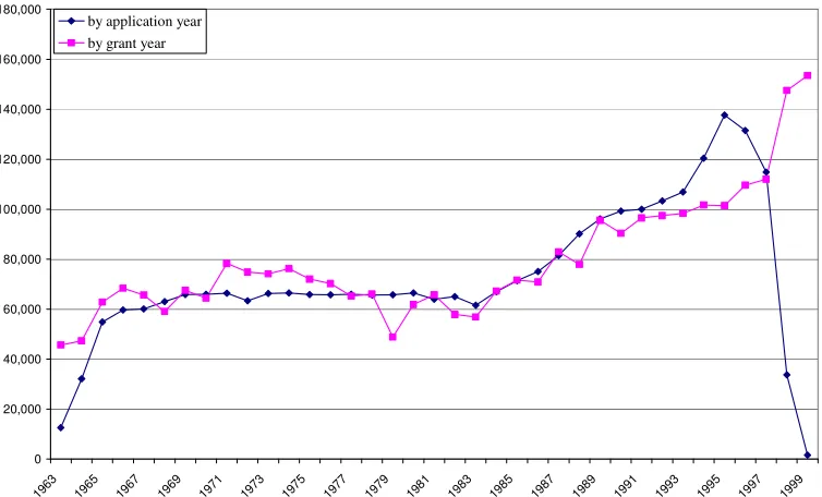
Using the framework developed above, this section provides a quantitative assessment on the effects of
eliminating blocking patents. Figure 1 shows that private spending on R&D in the US as a share of GDP
has been rising sharply since the beginning of the 80’s. Then, after a few years, the number of patents
granted by the US Patent and Trademark Office also began to increase rapidly as shown in Figure 2.
aggregate data of the US’s economy from 1953 to 1980 to examine the extent of R&D underinvestment
before these policy changes. The goal of this numerical exercise is to quantify the effects of eliminating
blocking patents on R&D and consumption.
3.1. Backloading Discount Factor
The first step is to calibrate the structural parameters and the steady-state value of the backloading
discount factor
ν
. The average annual TFP growth rateg
TFP is 1.33%,13 and the labor-force growth raten is 1.94%.14 The annual depreciation rate
δ
on physical capital and the household’s discount rate are set to conventional values of 8% and 4% respectively. For the aggregate markupµ
~=µ
1−θ, Laitner and
Stolyarov (2004) estimate that
µ
~ is about 1.1 (i.e. a 10% markup) in the data. For a givenµ
~, each valueof
θ
(i.e. the fraction of competitive industries in the intermediate-goods sector) corresponds to a uniquevalue for the industry markup
µ
in monopolistic industries, and I will consider a wide range of values for} 75 . 0 , 5 . 0 , 25 . 0 , 0
{ . . .
∈
θ
. A number of structural studies based on patent renewal models has estimatedthe arrival rate of innovations
λ
, and I will consider a reasonable range of values forλ
∈[0.04,.0.20]. 15For the capital intensity parameter in the R&D sector, I will set
β
=α
as the benchmark case.16For the remaining parameters {
ν
,α
,σ
}, the model provides three steady-state conditions for thecalibration: (a) R&D as a share of GDP; (b) labor share; and (c) the rate of investment in physical capital.
(54)
−
+
−
−
−
+
=
+
K K L
L r
r
s
s
s
s
Y
RK
wL
1
1
)
1
(
1
α
α
µ
θ
µθ
,
13
Multifactor productivity for the private non-farm business sector is obtained from the Bureau of Labor Statistics.
14
The data on the annual average size of the labor force is obtained from the Bureau of Labor Statistics.
15
For example, Lanjouw (1998) structurally estimate a patent renewal model using patent renewal data in a number of industries from Germany, and the estimated probability of obsolescence ranges 7% for computer patents to 12% for engine patents. Also, a conventional value for the rate of depreciation in patent value is about 15% (e.g. Pakes (1986)). In the current model, the patent-value depreciation rate is given by λ−gY, which implies that λ should be at least 15%. On the other hand, Caballero and Jaffe (2002) estimate a mean rate of creative destruction of about 4%.
16
(55) + − − − =
µ
θ
µθ
α
1 1 1 L s Y wL , (56)+
−
+
+
−
+
−
−
+
=
δ
α
σ
ρ
δ
α
µ
θ
µθ
α
)
1
/(
)
1
/(
)
1
(
)
1
(
. TFP TFP Kg
g
n
s
Y
I
,The average private spending on R&D as a share of GDP is 1.15%,17 and the labor share is set to a
[image:24.612.92.422.74.160.2]conventional value of 0.7. The long-run ratio of business investment to non-housing GDP is 14%.18
Table 1 presents the calibrated values for the structural parameters along with the real interest rate
) 1 /(
.
α
σ
ρ
+ −= gTFP
r and the industry markup
µ
(1.1)1/(1−θ)= for
θ
∈{0,.0.25,.0.5,.0.75} and] 20 . 0 , 04 . 0 [ . ∈
λ
.[insert Table 1 here]
Table 1 shows that the calibrated values for {
α
,σ
,r} are invariant to different values ofλ
for a givenvalue of
θ
. The calibrated value for the elasticity of intertemporal substitution (i.e. 1/σ
) is about 0.25,which is closed to the empirical estimates from econometric studies.19 The implied real interest rate is
about 11%, which is higher than the historical rate of return on the US’s stock market, and this higher
interest rate implies a lower optimal level of R&D spending and a higher steady-state value of the
backloading discount factor. As a result, the model is less likely to overestimate the extent of R&D
underinvestment and the degree of inefficiency from blocking patents. Re-expressing (55) into (58) shows
that
ν
decreases asλ
increases.(57)
λ
α
σ
ρ
µ
µ
θ
λ
ν
+ − − + − − − = ) 1 /( ) 1 ( / ) 1 )( 1 ( & TFP g n GDP D R . 17The data is obtained from the National Science Foundation and the Bureau of Economic Analysis. R&D is net of federal spending, and GDP is net of government spending. The observations in the data series of R&D spending are missing for 1954 and 1955.
18
Business investment refers to total private investment less investment in owner-occupied housing, and this data is obtained from Laitner and Stolyarov (2005).
19
Furthermore, the fact that the calibrated values of
ν
∈[0.169,.0.424] are very small suggests a severedegree of inefficiency from blocking patents in the economy. Therefore, eliminating blocking patents may
be an effective method to stimulate R&D. After calibrating the externality parameters and computing the
first-best level of R&D spending, the effects of eliminating blocking patents will be quantified.
3.2. Externality Parameters
The second step is to calibrate the values for the externality parameters
γ
(intratemporal duplication) andφ
(intertemporal spillover). For each value ofg
A,g
Z,n
,α
andβ
, the balanced-growth condition(50) determines a unique value for
γ
/(1−φ
), which is sufficient to determine the new balanced-growthlevel of consumption. However, holding
γ
/(1−φ
) constant, a largerγ
implies a faster rate ofconvergence to the new balanced-growth path; therefore, it is important to consider different values of
γ
.As for the value of
g
A, I will set gA =ξ
.gTFP forξ
∈[0,.1]. The parameterξ
captures the fraction oflong-run TFP growth that is driven by R&D, and the remaining fraction is driven by the exogenous
process Zt such that
g
Z=
(
1
−
ξ
)
g
TFP. Table 2 presents the calibrated values ofφ
for a subset of values forγ
∈[0.1,.1.0] andξ
∈[0,.1].[insert Table 2 here]
Table 2 shows that the calibrated values for
φ
are very similar across different values ofθ
implying thatthe first-best level of R&D spending and the extent of R&D over- or underinvestment are about the same
across different values of
θ
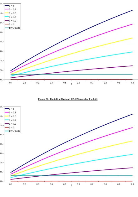
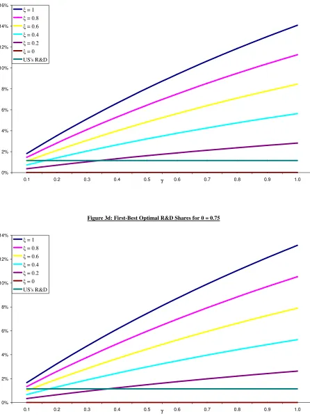
.3.3. First-Best Level of R&D Spending
This section calculates the first-best level of R&D share (1 ) * /(1 *) * /(1 * )
. K K
L
L s s s
s − + −
−
α
α
. Figure 3[insert Figure 3 here]
Figure 3 shows that there was underinvestment in R&D prior to 1980 over a wide range of parameters
unless
γ
andξ
are very small. Since it is difficult to determine the empirical value ofξ
, I will leave itto the readers to decide on their preferred values and continue to present results for a range of parameters.
3.4. Eliminating Blocking patents
Given the calibrated structural parameters, this section quantifies the effects of eliminating blocking
patents on R&D and consumption. Upon eliminating blocking patents (i.e. setting
ν
=1), the steady-stateshare of R&D given by
(
wL
r+
RK
r)
/
Y
would increase substantially to the values in Table 3. [insert Table 3 here]In the following, the effect of eliminating blocking patents is firstly expressed in terms of the percentage
change in the balanced-growth level of consumption per year. Along the balanced-growth path, per capita
consumption increases at an exogenous rate gc. Therefore, after dropping the exogenous growth path and
some constant terms and solving for the balanced-growth path of R&D technology and steady-state
capital-labor ratio, I derive the expression for the endogenous parts of long-run consumption as a function
of the steady-state value of the backloading discount factor
ν
through the capital investment rate i(ν
),and the R&D shares of capital and labor (where
s
r(
ν
)
=
s
L(
ν
)
=
s
K(
ν
)
becauseα
=β
).Lemma 3: For
α
=β
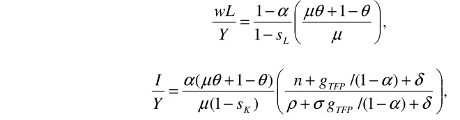
, the expression for the endogenous parts of consumption on the balanced-growth path is(58) = − − − − −
− −
− − −
− −
+ −
αγ φ α
φ αγ
φ α
γ βγ
φ α
γ β φ α
ν
ν
ν
ν
ν
(1 )(1 )) 1 ( )
1 )( 1 ( )
1 )( 1 (
) 1 (
0( ) i( ) (1 i( ))sr( ) (1 sr( ))
c .20
20
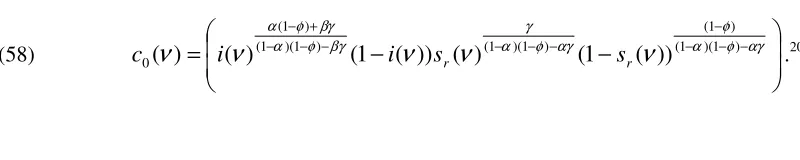
[image:26.612.73.473.598.678.2]Therefore, in the case of a change in
ν
, the percentage change in long-run consumption can bedecomposed into four terms.
(59)
− ∆ − − −
− +
∆ − − −
+ − ∆ + ∆
− − −
+ −
= ∆
)) ( 1 ln( )
1 )( 1 (
) 1 ( )
( ln )
1 )( 1 (
)) ( 1 ln( )
( ln )
1 )( 1 (
) 1
(
) ( ln 0
ν
αγ
φ
α
φ
ν
αγ
φ
α
γ
ν
ν
αγ
φ
α
γ
φ
α
ν
r
r s
s
i i
c .21
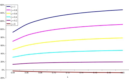
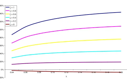
Figure 4 shows that eliminating blocking patents should have a substantial positive effect on long-run
consumption unless
ξ
is very small. Also, a back-of-the-envelope calculation shows that the change inconsumption mostly comes from
(
γ
/((
1
−
α
)(
1
−
φ
)
−
αγ
))
∆
ln
s
r(
ν
)
; in other words, other general-equilibrium effects only have secondary impacts on long-run consumption.[insert Figure 4 here]
After examining the effect on long-run consumption, the next numerical exercise computes the
entire growth path of consumption upon eliminating blocking patents. Figure 5a compares the transition
path (in blue) of log consumption per capita with its original balanced-growth path (in red) and its new
balanced-growth path (in green) for the following parameters {
ξ
,γ
,λ
,θ
,δ
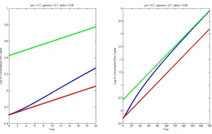
}={0.7,0.7,0.06,0,0.08} toillustrate the transition dynamics. Then, I will discuss the effects of changing these parameter values.
[insert Figure 5a here]
Upon setting
ν
=
σ
1=
1
, consumption per capita gradually rises towards the new balanced growth path. Although factor inputs shift towards the R&D sector and the output of final goods drops as a result, thepossibility of investing less and running down the capital stock enables consumption smoothing. To
compare with previous studies, such as Kwan and Lai (2003), Figure 5b presents the transition dynamics
for {
ξ
,γ
,λ
,θ
,δ
}={0.7,0.7,0.06,0,1} as an approximation to a model with no capital accumulation. Inthis case, the result is consistent with Kwan and Lai (2003) that consumption falls in response to the
21
[image:27.612.75.509.125.198.2]strengthening of patent protection. In this case, consumption falls by about 5% on impact and only
recovers to its original growth path after 3 years.
[insert Figure 5b here]
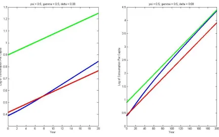
To ensure the robustness of this finding, a sensitivity analysis has been performed for different
values of
ξ
andγ
. At a larger value of eitherξ
orγ
, consumption increases by even more on impact.A larger
ξ
also implies a higher position of the new balanced-growth path. Holdingξ
constant, a largerγ
implies a faster rate of convergence. When bothξ
andγ
are small than 0.7, the household suffersconsumption losses during the initial phase of the transition path. For example, Figure 5c presents the
transition dynamics for {
ξ
,γ
,λ
,θ
,δ
}={0.5,0.5,0.06,0,0.08}.[insert Figure 5c here]
However, Figure 5d shows that when
ξ
is closed to one,γ
could be as small as 0.5 without causing anyshort-run consumption losses.
[insert Figure 5d here]
In summary, reallocating resources from the production sector to the R&D sector does not always lead to
short-run consumption losses. Finally, at a larger value of
λ
, the calibrated value forν
becomes smaller(see Table 1). This larger magnitude of the policy shock renders the algorithm unable to achieve
convergence when
ξ
andγ
are large. However, when the magnitude of the policy is small (e.g.ν
increases from 0.5 to 1), convergence is always achieved.
4. Conclusion
This paper has attempted to accomplish three objectives. Firstly, it develops a tractable framework to
model the transition dynamics of an economy with patent breadth and blocking patents in a generalized
quality-ladder growth model. Secondly, it identifies a dynamic distortion on capital accumulation that has
been neglected by previous studies on patent policy. Thirdly, it applies the model to the aggregate data to