Simulation based approach for measuring concentration risk

Munich Personal RePEc Archive

Simulation based approach for measuring

concentration risk

Kim, Joocheol and Lee, Duyeol

1 February 2007

Simulation based approach for measuring

concentration risk

April, 2007

Joocheol Kim

School of Economics, Yonsei University, 134 Shinchon-dong, Seodaemun-ku, Seoul,

120-749, Korea

Duyeol Lee

School of Economics, Yonsei University, 134 Shinchon-dong, Seodaemun-ku, Seoul,

120-749, Korea

Abstract

Asymptotic Single Risk Factor (ASRF) model is used to derive the regulatory

capital formula of Internal Ratings-Based approach in the new Basel accord

(Basel II). One of the important assumptions in ASRF model for credit risk is that

the given portfolio is well diversified so that one can easily calculate the required

capital level by focusing only on systematic risk. In real world, however,

idiosyncratic risk of a portfolio cannot be fully diversified away, causing the so

called concentration risk problem. In this paper we suggest simulation based

approach for measuring concentration risk using bank capital dynamic model.

This approach is especially suitable for a portfolio with relatively small to

medium number of obligors and relatively large sized loans.

Keywords: Basel II, ASRF model, credit risk, concentration risk

JEL Codes: G32, G33, G38

∗ _{Corresponding author}

Email addresses : [email protected] (Joocheol Kim) [email protected] (Duyeol Lee). Tel : +82-2-2123-5498 (Joocheol Kim)

Simulation based approach for measuring

concentration risk

1. Introduction

In recent years, many important advances have been made in modeling credit risk of

a portfolio. One of them is Asymptotic Single Risk Factor (ASRF) model, which is used

to derive the regulatory capital formula of Internal Ratings-Based approach in the new

Basel accord (Basel II).

Under the ASRF framework there are only two sources of risk, systematic risk and

idiosyncratic risk. As the number of obligors in a portfolio increases, idiosyncratic risk

is diversified away, so its contribution to portfolio risk disappears. Thus, one can easily

calculate required capital level by focusing only on systematic risk under the ASRF

assumptions. In real world, however, a bank’s portfolio is often not sufficiently

diversified. The fact that there are some large exposures in the portfolio implies that

there is a residual of undiversified idiosyncratic risk in the portfolio. Under these

circumstances, IRB formula in the Basel accord underestimates the required regulatory

capital. Some historical examples such as insolvency of Enron, Worldcom and Parmalat

show the dangers of misunderstanding concentration risk.1

The approaches for measuring concentration risk suggested in recent studies can be

categorized into two different types. The first approach is to adapt indices of

concentration such as Gini coefficient or Herfindahl-Hirschman Index (HHI). This

approach is simple and easy to perform. While these indices could be good measures for

concentration itself, they do not seem to serve well for concentration risk because they

do not take distribution of different quality obligors into consideration. The second

approach is granularity adjustment suggested by Gordy (2003). Its difficulties in

implementation and huge data requirement make it hard to be performed in practice.

Usually practitioners use both approaches to measure the concentration risk of their

portfolio. While the concentration measurement index such as HHI could not measure

the actual risk accurately, granularity adjustment sometimes overestimates the actual

concentration risk of a portfolio.

In this paper, we introduce a simulation based approach to measure concentration

risk. We show that HHI could not provide enough information to measure the actual

concentration risk. With the proposed approach, we are able to calculate the amount of

required capital for concentration risk directly. We believe that the approach is

especially suitable for banks with portfolios of relatively small number of obligors with

relatively large size of loans.

This paper is organized as follows. In section 2, we present detailed descriptions of

concentration risk and Herfindahl-Hirshman Index, respectively. Section 3 explains the

frameworks of our simulation based approach to measure concentration risk. Section 4

provides some numerical results based on the actual example and explains the

implication of those numbers. Section 5 concludes the paper.

2. Concentration risk under Basel II framework

2.1 The IRB model and concentration risk

In this section, we provide a brief summary on the key assumptions of the

Asymptotic Single-Risk Factor (ASRF) model that is used to calculate the regulatory

capital requirement by Basel II. In the risk factor model frameworks that underpin the

Internal Ratings-Based (IRB) risk weights of Basel II, credit risk of a portfolio is caused

by two main sources, systematic and idiosyncratic risks.2

Systematic risk represents the effect of unexpected changes in macroeconomic and

financial market conditions on the performance of borrowers. Borrowers may differ in

their degree of sensitivity to systematic risk, but few firms are completely indifferent to

the wider economic conditions in which they operate. Therefore, the systematic

component of portfolio risk is unavoidable and only partly diversifiable. Meanwhile

idiosyncratic risk represents the effects of risks that are particular to individual

borrowers. As a portfolio becomes more fine-grained, in the sense that the largest

individual exposures account for a smaller share of total portfolio exposure,

idiosyncratic risk is diversified away at the portfolio level. This risk is totally eliminated

in an infinitely granular portfolio (one with a very large number of exposures) as

unsystematic risk vanishes in Capital Asset Pricing Model.

The ASRF model framework underlying the IRB approach is based on two key

assumptions. The first one is that bank portfolios are perfectly fine-grained and the

second one is that there is only one source of systematic risk. When these two

assumptions hold, one can easily calculate required capital level depending on only one

systematic risk. In case of well diversified portfolio, the capital required for a loan does

not depend on the portfolio it is added to. This simplicity makes the new IRB

framework applicable to a wider range of countries and institutions. However, if any of

two assumptions is violated, there is no guarantee that the IRB approach and ASRF

model will be accurate. The violation of the assumption of the fine-grained portfolio

leads to concentration risk problem. Concentration of exposures in credit portfolios

arises from imperfect diversification of idiosyncratic risk in the portfolio. The small to

medium size of credit portfolio or some large exposures to specific individual obligors

can lead to concentration risk.

2.2 Herfindahl-Hirshman Index

The Herfindahl-Hirshman index3 (HHI), better known as the Herfindahl index, is a

statistical measure of concentration. The HHI accounts for the number of firms in a

market, as well as concentration, by incorporating the relative size of all firms in a

market. It is calculated by squaring the market shares of all firms in a market and then

summing the squares, as follows:

∑

= n

i i

MS HHI

1

2

)

( , (1)

where MS_i is market share of i th firm and n is the number of firms.

Well-diversified portfolios with a very large number of very small firms have an

HHI value close to zero whereas heavily concentrated portfolios can have a

considerably higher HHI value. In the extreme case of a monopoly, the HHI takes the

value of one.

In the context of the measurement of concentration risk, the HHI formula is

included as a main component of a number of approaches. But HHI itself has some

drawbacks to be used for measuring concentration risk. At first, it does not consider

distribution of exposures across credit ratings, so portfolios with the same HHI values

can have different sizes of concentration risks. Secondly, it does not allow concentration

risk to be expressed directly as economic capital, so it needs additional functions to

3 _{Board of Governors of the Federal Reserve System (1993): The Herfindahl-Hirshman}

calculate economic capital for concentration risk.

3. Framework for simulations

In this section, We introduce the framework for simulations presented in Peura and

Jokivuolle(2003) and how to use this bank capital dynamics model to calculate

concentration risk.

3.1 Bank capital dynamics based on rating transitions

To model bank capital dynamics and required capital buffers and to avoid confusion

of notations, we use three different types of bank capital, the actual capital, the

regulatory capital and the economic capital. The actual capital is bank’s actual capital

and denoted by . The regulatory capital is the minimum regulatory capital charge of

Basel II and denoted by . And the economic capital is minimum capital level

calculated by bank without considering regulatory capital. Now let there be a bank with

assets consisting of illiquid corporate loans. Under Basel II framework, the actual bank

capital must satisfy equation (2).

t

A

t

R

t

t R

A ≥ (2)

Equation (2) gives us intuition how to determine initial actual capital of a bank. By

calculating required initial actual capital subject to equation (2), we can have the

required capital amount for credit risk of a portfolio.

Now, to model bank’s actual capital dynamics, we assume that the bank’s profit

occurs before credit losses during period t. The bank’s credit loss during period t is

denoted by and the dividends paid out of the bank capital at time t by , the issues

of new equity at time t by . Now, the bank’s capital dynamics can be determined by

t

L V_t

t

S

1 1 1 1

1 + + + +

+ = t + t − t − t + t

t A I L V S

A . (3)

The bank determines the actual capital level preparing for severe macroeconomic

downturns. In those conditions when capital is insufficient, it is natural to assume that

equity. So, with little loss of generality, we can assume that both the and the

terms in equation (3) equal zero in all scenarios. Now we can express the capital

dynamics that we simulate as

1

+

t

V S_t+1

1 1

1 + +

+ = t + t − t

t A I L

A (4)

By rolling the difference equation (4) forward, we can get the capital at time t from

∑

∑

= =

− +

= t

s s t

s s

t A I L

A

1 1

0 (5)

The equation (5) implies that the bank’s capital dynamics are determined by two

stochastic factors, the cumulative net profit and the cumulative change in the minimum

capital requirement. Now, we need to model bank income, credit losses and regulatory

capital in order to simulate the dynamics of a bank’s capital. The bank income and

credit losses depend on rating transitions because they depend on default events of

obligors. Obligors’ defaults can be simulated based on rating transitions model. And

also regulatory capital can be simulated by rating transitions because IRB formula of

Basel II needs credit ratings of obligors as a component. In Peura and Jokivuolle (2003),

they used a one-factor version of the CreditMetrics™ framework (J.P. Morgan, 1997) as

rating transitions, extended with an underlying conditioning variable which is

interpreted as business cycle state. The Creditmetrics model takes the transition

probability matrix of ratings as given, which is determined by the business cycle state in

Peura and Jokivuolle (2003). In particular, they assume that the business cycle variable

is a two-state, time homogenous, Markov Chain, whose possible states are ‘expansion’

and ‘recession’. In Bangia et al.(2002), they used models of ratings dynamics of this

type.

Credit portfolio models are typically implemented as one-period simulations with an

annual horizon. However, because banks in most countries report their capital adequacy

to their regulators quarterly, multi-period simulations of rating changes should be

performed in quarterly time increments. Both the rating transition probabilities and the

regime transition probabilities in this simulation are quarterly probabilities estimated

based on US data. The conditional transition matrices for the expansion and the

recession states are from Bangia et al.(2002), which are based on Standard and Poor’s

data on US corporate ratings over the period 1981-1998. The regime switching

1959-1998. The stationary distribution of the business cycle state implied by this transition

matrix is (79%, 21%).

Now we will explain how the evolution of ratings in this model determines bank

income, credit losses. For convention of notations, we define an indicator variable

which assigns 1 when i th obligor of the bank’s portfolio defaults at time t, otherwise 0.

t i D_, , , 1 ( 0 i t i t

with probability PD k D otherwise ⎧ ⎨ ⎩ ) , ) i t

, (6)

where unconditional default probability corresponding to rating by .

Regulatory capital is determined by the capital charge function of Basel II and rating

transitions. Bank income is determined by interests of loans and usually interests are

determined directly proportional to expected loss of loans. Credit losses are determined

by default events. Using these properties, we can express the variables , and

defined earlier equations in terms of the following sums over obligors in the bank’s

portfolio:

, i t

k PD k( i t_, )

t

R I_t L_t

, 1

( ( ) ) ( 1

n

t i t i

i

R f PD k EAD D

=

=

∑

, i t

, (7)

, 1

( ) ( 1 )

n

t i i t i

i

I β LGD PD k EAD D

=

=

∑

, , 1

1

(

n

t i i i t

i

L LGD EAD D D ₋

=

=

∑

where is the capital charge function of Basel II, which takes the default

probability as an argument. is the credit rating of obligor at time t. is

the nominal exposure of obligor . )

(⋅

f

t i

k_, i EAD_i

i β is a parameter which indicates the ratio of the

nominal loan margin to the expected loss rate (the unconditional default probability

times the loss given default percentage) in the portfolio. is the loss given default

to nominal exposure ratio. is the number of obligors in the bank’s portfolio at time 0.

Formula (9) implies that the bank earns income as a fixed multiple of its unconditional

expected loss rate.

i

LGD

n

We assume that the underlying asset value correlations, which together with the

transition probabilities determine the rating transition correlations, do not depend on the

correlation formula of Basel II.

Now, we have bank’s capital dynamics and this result must satisfy equation (2). For

convenience of notation, we define capital buffer , which is the difference between

the bank’s actual capital and the regulatory capital. It can be interpreted as capital buffer

to absorb the risk from uncertainty and given by

t

B

t t

t A R

B = − (10)

Holding capital buffer means an opportunity cost for banks. In this point of view,

requiring equation (2) to hold in all possible states of the world is not economical to the

bank. Therefore banks use value-at-risk type probabilistic regulatory capital requirement

to calculate the size of capital buffer. Value-at-risk is defined as the α th percentile of

the distribution and the constraint of VaR can be expressed as

0mint T t 0

P B α

≤ ≤

⎡ _≥ ⎤ _≥

⎣ ⎦ , (11)

where α is a confidence level associated with regulatory capital adequacy, such as

99% or 99.9%. The dynamics of depend on the initial capital buffer because

is increasing in . By substituting equation (5) into equation (10), and applying

the inequality (2), we can express the regulatory capital requirement at time t:

t

B B₀

t

B B₀

0

0 1

1

0 + − − + ≥

=

∑

∑

t (12)

Here the capital buffer at time t is expressed in terms of the initial capital buffer, the

inflows and outflows of capital between time 0 and time t, as well as the change in the

regulatory capital charge R_t between time t and time 0. In particular, is the capital charge associated with the bank’s initial portfolio evaluated based on ratings of the

assets in the portfolio at time t. By simulation based on capital dynamics explained

above, we can calculate a minimum value for which satisfies equation (12) and we

denote it with

t R 0 B 0 ˆ

B . The required initial capital buffer Bˆ₀ is given by

{

}

0 0 ₀

ˆ _{inf : min 0}

t t T

B B P B α

≤ ≤

⎡ ⎤

Now, by assuming that equation (13) determines the capital buffer, we can calculate

initial bank capital as

0 0

ˆ ˆ

0

A =R +B , (14)

where Aˆ₀ is required initial capital for credit risk of a loan portfolio.

3.2 Measuring concentration risk

Simulations based on bank capital dynamics model introduced in previous section

provide required capital minimum level directly from distribution of bank’s initial actual

capital. However, in this paper, we need additional simulation and model extensions to

calculate concentration risk. Any given portfolio, there exist a benchmark portfolio

which have no concentration. Now using simulations, we can calculate required initial

capital levels for these two portfolios, real one and benchmark case. The difference

between these two values is additional required capital caused by concentration in the

real portfolio. In Peura and Jokivuolle(2003), they form portfolios according the given

quality distributions that each have 100 equal sized loans to stress test bank capital

adequacy. In this framework, there is no concentration in the portfolio. It is not only

unrealistic but also unsuitable for our main goal which is to calculate concentration risk.

Therefore, we form portfolios which have differently sized loans. In order to perform

the simulation, we need business cycle scenarios. In Peura and Jokivuolle(2003), they

used various assumptions concerning the initial business cycle state as well as the

duration of recessions. But we used randomly selected scenarios because the main

purpose of our model is just to calculate the VaR type criterions from the distributions.

3.3 Testing Herfindahl-Hirschman Index

In the context of the measurement of concentration risk, the HHI formula is

included as a main component of a number of approaches. But there are two types of

shortcomings of HHI to be used for measuring concentration risk. Firstly, HHI doesn’t

take quality of a portfolio into consideration. It implies that the portfolios differently

distributed across the credit ratings can have the same HHI. In the next section, we form

portfolios have different sizes of concentration risk. Secondly, HHI doesn’t reflect

location of concentration in a portfolio. Even though distributions of loans in portfolios

are same, the locations of concentration can differ. If the sizes of loans in portfolios are

same, then they still have same HHI regardless the locations of concentration. It means

the portfolios that have concentrations in different credit ratings can have same HHI. To

show this we form two portfolios which have same distribution of loans across the

credit ratings but have concentrations in different grades and also show these portfolios

have different sizes of concentration risk in the next section.

4. Numerical Results

Our simulations results are calculated by following steps. First, we form two sets of

portfolios. Second, we determine business cycle scenarios. Last, we perform

Monte-Carlo simulations based on bank capital dynamics described above.

We present our main results subject to the following base case parameters: portfolio

maturity T equal to 2.5 years, a bank income equal to the unconditional expected credit

loss(β =1), an loss given default of 45% across all obligors( ), and a

confidence level

0.45

i

LGD =

α of 99%. We use 1,000 scenarios selected randomly. The number of simulations is 1,000 for each scenario. So we have 1,000,000 samples.

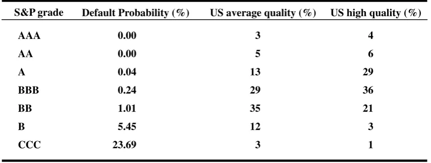
We take representative portfolios of banks from a Federal Reserve Board survey as

reported by Gordy(2000). The portfolios are reported in Table 1.

Table 1. Average bank portfolios

AAA

AA

A

BBB

BB

B

CCC

0.00

0.00

0.04

0.24

1.01

5.45

23.69

3

5

13

29

35

12

3

4

6

1 3 21 36 29

US high quality (%) US average quality (%)

S&P grade Default Probability (%)

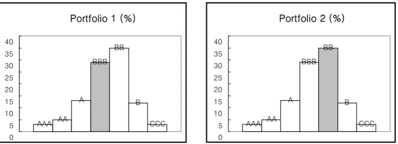
These distributions of portfolios do not reflect concentration because they are

calculated using exposure based data. In the first case, we form two portfolios using US

average quality portfolio and two portfolios using US high quality portfolio. In each

case, the benchmark portfolios have the distributions that each obligor has same

nominal exposure. Portfolio 1 has concentration in credit rating of BB of average

quality portfolio. Portfolio 2 has concentration in the same grade of high quality

portfolio. In order to eliminate the effect of location of concentration, we let both

portfolios have concentrations in the same grades.

Portfolio 1

AAA AA A

BBB BB

B

CCC

0 5 10 15 20 25 30 35 40

Portfolio 2

40 35

0 5 10 15 20 25 30

AAA AA A

BBB

BB

B CCC

Fig. 1. The distributions of portfolio 1 and 2. Each portfolio has concentration in shaded

area.

These two portfolios have two obligors which have exposures of about 10% out of

total portfolio exposures. And two portfolios have the same HHI (0.272). Table 2 shows

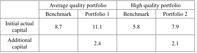
the main result of simulations.

Table 2. Initial actual capitals of portfolios (%)

Average quality portfolio High quality portfolio

Benchmark Portfolio 1 Benchmark Portfolio 2

Initial actual

capital 8.7 11.1 5.8 7.9

Additional

capital 2.4 2.1

The differences between each portfolio and benchmark portfolio are additional

required capitals arise from concentration. It can be interpreted as additional risks from

risk of portfolio 2 is 2.1%. The difference 0.3% is large enough to conclude that the

concentration risk from differently distributed portfolios with same HHI can be different.

In the second case, we form three portfolios using US average quality portfolio. The

benchmark portfolio has the distribution that each obligor has same nominal exposure.

Portfolio 1 has concentration in credit rating of BBB. Portfolio 2 has concentration in

BB.

Portfolio 2 (%)

AAA AA A

BBB BB

B

CCC

0 5 10 15 20 25 30 35 40 Portfolio 1 (%)

AAA AA A

BBB BB

B

CCC

0 5 10 15 20 25 30 35 40

Fig. 2. The distributions of portfolio 1 and 2. Each portfolio has concentration in shaded

area.

These two portfolios have two obligors which have exposures of about 10% out of

total portfolio exposures. And two portfolios have the same HHI (0.272). Table 3 shows

the main result of simulations.

Table 3. Initial actual capitals of portfolios (%)

Benchmark Portfolio 1 Portfolio 2

Initial actual capital 8.7 10.3 11.1

Additional capital 1.6 2.4

In this case, the additional risk of portfolio 1 is 1.6% and the additional risk of

portfolio 2 is 2.4%. The difference 0.8% is large enough to conclude that the

concentration risk from portfolios that have concentrations in different grade with same

HHI can be different.

In order to show the problems caused by using HHI for concentration risk measure

more clearly, we form 1000 randomly selected portfolios(with HHI from 0.012~0.015)

risk. Using simple linear regression, we found R2equal to 0.043. It implies that HHI could not provide enough information to measure the actual concentration risk.

Fig. 3. Scatter diagram for Herfindahl-Hirschman Index and concentration risk of

average quality portfolio

5. Conclusion

This paper provides a simulation based approach to measure concentration risk. In

addition, it is shown that Herfindahl-Hirshman Index can not be a good measure for

concentration risk. Given bank capital dynamic model, simulations directly provide the

amount of required capital for concentration risk of a loan portfolio while more simple

methods such as HHI or Gini coefficient need an additional function. And also it

provides more precise result, compared with approximation methods such as granularity

adjustment. It might be more time-consuming than other methods, but it is still the

better way especially for banks with portfolios of relatively small number of obligors

References

Bangia, A, Diebold, F, Kronimus, A, Schagen, C, Schuermann, T(2002): “Ratings

migration and the business cycle, with application to credit portfolio stress testing,

Journal of Banking and Finance, vol 26, pp 445-474.

Basel Committee on Banking Supervision(2001): The new Basel capital accord,

consultative document, Basel, January.

(2003): The new Basel capital accord, consultative document, Basel, April.

(2006): International convergence of capital measurement and capital

standards: a revised freamework, comprehensive version, Basel, June.

(2006): Studies on credit risk concentration, working paper, Basel, November.

Board of Governors of the Federal Reserve System (1993): The Herfindahl-Hirshman

Index, Federal Reserve Bulletin, March, pp 188-189

Deutsche Bundesbank(2006): Concentration risk in credit portfolios, monthly report,

June.

Emmer, S and D Tasche(2003): “Calculating credit risk capital charges with the

one-factor model”, Journal of Risk, vol 7, no 2, pp 85-101.

Gordy, M(2000): “A comparative anatomy of credit risk models, Journal of Banking and

Finance, vol 24, pp 119-149.

Gordy, M and E Lutkebohmert(2004): “Granularity adjustment in portfolio credit risk

measurement”, in G Szego(ed), Risk measures for the 21st Century, Wiley.

J.P. Morgan(1997): CreditMetrics™ - Technical Document, J.P. Morgan, New York

Peura, S and Jokivuolle, E(2003): “Simulation based stress tests of banks’ regulatory

capital adequacy”, Journal of Banking & Finance, vol 28, pp1801-1824.