Simulated Evidence on the Distribution of the Standardized One Step Ahead Prediction Errors in ARCH Processes

Munich Personal RePEc Archive

Simulated Evidence on the Distribution

of the Standardized One-Step-Ahead

Prediction Errors in ARCH Processes

Degiannakis, Stavros and Xekalaki, Evdokia

Department of Statistics, Athens University of Economics and

Business, Greece, Department of Statistics, University of California,

Berkeley CA, USA

2007

Online at

https://mpra.ub.uni-muenchen.de/96326/

Simulated Evidence on the Distribution of the Standardized One-Step-Ahead

Prediction Errors in ARCH Processes

*

Stavros Degiannakis

Adjunct Lecturer

Department of Statistics, Athens University of

Economics and Business, Greece. Tel.: +30-210-8203-120

FAX.: +30-210-2614-644 E-mail address: [email protected]

and

Adjunct Assistant Professor

Department of Informatics and Biomedicine, University of Central Greece, Lamia.

Tel.: + 30-223-1066-700 Fax.: +30-223-1066-715 Corresponding Author

Evdokia Xekalaki

Professor

Department of Statistics, Athens University of

Economics and Business, Greece. Tel.: +30-210-8203-269

Fax.: +30-210-8238-798 E-mail address: [email protected]

and

Department of Statistics, University of

California, Berkeley CA, USA. Tel.: +510-642-2781

Fax.: +510-642-7892

ABSTRACT

In statistical modeling contexts, the use of one-step-ahead prediction errors for testing hypotheses

on the forecasting ability of an assumed model has been widely considered. Quite often, the testing procedure requires independence in a sequence of recursive standardized prediction errors,

which cannot always be readily deduced particularly in the case of econometric modeling. In this paper, the results of a series of Monte Carlo simulations reveal that independence can be assumed

to hold.

Index terms: ARCH models, Monte Carlo Simulation, One-step-ahead Prediction Errors,

Predictability, Standardized Prediction Error Criterion.

*

I. INTRODUCTION

Defining a standardized prediction error criterion (SPEC), Degiannakis and Xekalaki (2005a)

proposed a model selection algorithm for ARCH models. The algorithm allows switching from

the model used at time t1 for forecasting volatility to another model for use at time

t

and, in particular, to the model with the minimum value of the average squared standardized prediction error. As indicated by the results obtained by Degiannakis and Xekalaki (2005b), the SPEC model selection procedure appears to have a satisfactory performance in selecting the model that

generates better volatility predictions. Moreover, the SPEC algorithm exhibited a satisfactory performance on a simulated options market (Xekalaki and Degiannakis 2005) as well as on

trading S&P500 options on a daily basis (Degiannakis and Xekalaki 2001). The general finding is that the prediction performance improves if one switches models over time. In particular,

switching from one model to another governed by the SPEC model selection rule appears to lead to a superior predictive performance. The reason might be traced in that jumping from one model

to the other according to SPEC reflects a sort of a procedure adapting to the changes of the marketplace. However, model selection procedures based on standardized one-step-ahead

prediction errors often require independence in a sequence of recursive standardized prediction errors, which cannot always be readily deduced particularly in the case of econometric modeling.

In this paper, on the basis of the results of a series of Monte Carlo simulations, it is conjectured that independence holds. A theoretical justification can be found in Degiannakis and Xekalaki (2005a).

II. THE ARCH PROCESS

An ARCH process, t, is presented as:

 



, ,..., , ,...



1 , 0 ~

2 1 2 1 2

. . .

   





t t t t t

d i i t

t t t

g

N z

z

    

 

(1)

where zt is a sequence of independently and identically distributed random variables, with

autocorrelation, Cor



zt,zt



, approximately





1

, 0T

N distributed, t is a time-varying, positive

measurable function of the information set at time t1 and g



. could be a functional form that

has been presented in the ARCH literature.

Since very few financial time series have a constant conditional mean of zero, an ARCH

model can be presented in a th _{order autoregressive form by letting} t

 be the innovation process









 



, ,..., , ,...



1 , 0 ~ , 0 ~ | 2 1 2 1 2 . . . 2 1 1           



t t t t t d i i t t t t t t t t i i t i t g N z z N I y c y            (2)

The most commonly used conditional variance function is the GARCH(1,1)

model: 2 1 1 2 1 1 0 2    

 _{t t}

t a a b

 .

A wide range of proposed ARCH models is covered in surveys such as Bollerslev et al. (1994) and Degiannakis and Xekalaki (2004).

III. SIMULATION OF THE AR(1)GARCH(1,1)PROCESS

In the sequel, a Monte Carlo simulation is used to provide evidence for the assumption of independently and identically distributed standardized one-step-ahead prediction errors. The

procedure consists of three stages:

1. _{Generate data from the AR(1)GARCH(1,1) process}

 Generate a series of 32000 values from the standard normal distribution, i.e. z .~. .N

 

0,1 d i i

t .

 Generate an equal number of values

 

32000 1

 t t

 of the innovation ARCH process, by

multiplying the collection

 

32000 1

 t t

z by a specific conditional variance form, or 2

t t

t z 

  , for

2 1 2 1 2 8 . 0 12 . 0 0001 .

0    

 _{t t}

t  

 .

 Generate a first order autoregressive processes, yt 0.06yt1t, for the conditional mean,

based on the values

 

32000 1

 t t

 of the innovation process.

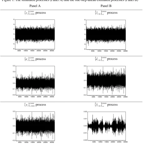
Panel A of Figure 1 plots the simulated processes while panel A of Table 1 presents the relevant

descriptive statistics. According to results obtained in literature (e.g. Engle and Mustafa 1992),

the shocks to the variance, Et

 

t Et

 

t  t  t vt

2 2 2 1

2   

 , generate a martingale difference

sequence. These shocks are neither serially independent nor identically distributed. According to

the Brock et al.’s (1996) BDS test for independence only the process defined by zt is

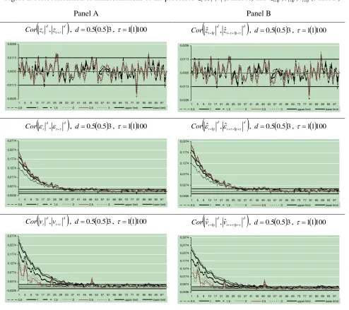
independently distributed. The test is presented for two correlated dimensions but it has been computed for higher values and the results are qualitatively unchanged. Panel A of Figure 2

presents the autocorrelation of transformations of the processes defined by zt,vt,t . The

half-length of the 95% confidence interval for the estimated sample autocorrelation equals

0113 . 0 / 96 .

1 T  , in the case of a process with independently and identically normally distributed

components. On the other hand, the processes defined by vt and t are autocorrelated in half of

GARCH(1,1) process and Karanasos (1999) extends the results to the GARCH(p,q) model. He

and Teräsvirta (1999) derive the autocorrelation function of the squared and absolute errors for a

family of first order ARCH processes.

2. _{Estimate the parameters of the AR(1)GARCH(1,1) model}

 The AR(1)GARCH(1,1) model is applied, for the data produced from the

AR(1)GARCH(1,1) process. Dropping out the first 1000 data, maximum likelihood estimates of

the parameters are obtained by numerical maximization of the log-likelihood function, using a rolling sample of constant size equal to 1000. At each of a sequence of points in time, the

maximum likelihood parameter vector, ˆt 



cˆ1,t,aˆ0,t,aˆ1,t,bˆ1,t



, is being estimated in order to compute

the conditional mean and variance:

t t t

t c y

yˆ_1| ˆ_1,

2 | , 1 2 | , 1 , 0 2 |

1 ˆ ˆ ˆ

ˆt t a t attt bttt

    .

(3)

3. _{Compute the standardized one-step-ahead prediction errors,}





1

| 1 | 1 1 |

1 ˆ ˆ

ˆ 

  

t  t  t t t t

t y y

z 

According to Degiannakis and Xekalaki (2005a), under the assumption of constancy of

parameters over time,

   

ˆt ˆt1 ...

   

ˆT ˆ , the estimated standardized one-step-ahead

prediction errors zˆt1|t,zˆt2|t1,...,zˆT1|T are asymptotically independently standard normally distributed.

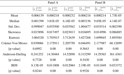
 The one-step-ahead estimated processes are presented in Panel B of Figure 1, while Panel B of Table 1 presents the relevant descriptive statistics. According to the tests of normality and

independence, the one-step-ahead standardized prediction error process,





1 | 1 | 1 1 |

1 ˆ ˆ

ˆ 

  

t  t  t t t t

t y y

z  , is

independently normal distributed. Moreover, if zˆ 1| .~..N

 

0,1 d i i t

t , then



  T t t t z 1 2 | 1

ˆ should be chi-square

distributed with T degrees of freedom, and mean and variance:

T z E T t t t 

  

_

  1 2 | 1

ˆ and V z T

T t t t 2 ˆ 1 2 | 1

  

_



 . (4)

According to Table 2, which presents the descriptive statistics of



  T t t t z 1 2 | 1

ˆ , the processes are

chi-square distributed in all the cases. Moreover, if zˆt1|t is a sequence of i.i.d. variables then the

autocorrelation of any transformation of zˆt1|t,





d t t d t t z z

Cor ˆ_1| , ˆ_1|_ , d0, is





1

, 0T

N distributed.

Panel B of Figure 2 presents the autocorrelation of transformations of the processes zˆt1|t,ˆt1|t,vˆt1|t.

Since the sum of squared standardized one-step-ahead prediction errors is chi-square distributed,

and the transformations of zˆt1|t are not autocorrelated, our findings point towards the

IV. SIMULATION OF THE GARCH,EGARCH AND TARCH PROCESSES

In the sequel, the assumption that the standardized one-step-ahead prediction errors are

independently and identically distributed is investigated for higher order of autoregressive processes for the conditional mean and conditional variance functions of the following types: The GARCH(p,q) model, Bollerslev (1986):





_







       p i i t i q i i t i

t a a b

1 2 1

2 0

2  

 . (5)

The EGARCH(p,q) model, Nelson (1991):

 

_

_



 



       _                  p i i t i q

i t i

i t i i t i t i

t a a b

1 2 1 0 2 ln ln      

 . (6)

The TARCH(p,q) model, Glosten et al. (1993):





_







          p i i t i t t q i i t i

t a a d b

1 2 1 2 1 1 1 2 0

2    

 , (7)

where dt 1 if t 0, and dt 0 otherwise.

The procedure followed is comprised of the following steps:

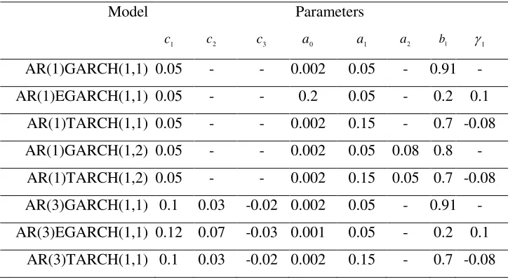
1. Eight processes have been generated with coefficients presented in Table 3

2. Estimate the parameters of the simulated processes

 At each of a sequence of points in time, the maximum likelihood parameter vector



t t t t t t t t



t cˆ1,,cˆ2,,cˆ3,,aˆ0,,aˆ1,,aˆ2,,bˆ1,,ˆ1,

ˆ 

  is being estimated. The models are estimated 30000 times and

the conditional mean and variance are computed in (8)-(11):

The th

order Autoregressive process:







      1 1 , | 1 ˆ ˆ i i t t i t

t c y

y . (8)

The GARCH(1,q) model:





2

| , 1 1 2 | 1 , , 0 2 |

1 ˆ ˆ ˆ

ˆ t tt

q i t i t t i t t

t a a  b 

  







 

 . (9)

The EGARCH(1,1) model:

 

_                    2 | , 1 | | , 1 | | , 1 , 0 2 |

1 exp ˆ ˆ ˆ ˆ ln

ˆ t tt

t t t t t t t t t t t t

t a a  b 

  



 _{. (10)}

The TARCH(1,q) model:





2

| , 1 2 | , 1 1 2 | 1 , , 0 2 |

1 ˆ ˆ ˆ ˆ

ˆ q _{t tt t t tt}

i t i t t i t t

t a a    d b 

  



 



 

 . (11)

3. Compute the standardized one-step-ahead prediction errors





1

| 1 | 1 1 |

1 ˆ ˆ

ˆ 

  

t  t  t t t t

t y y

z 

independently and identically distributed standardized one-step-ahead prediction errors in this

case too.

Finally, one more set of GARCH(1,1) processes is simulated in order to investigate if

changes in the coefficients affect the distribution of zˆt1|t. We generate a series

 

20000 1

 t t

 of 20000

values for each of 18 innovation GARCH(1,1) processes by multiplying the generated values of

t

z by _t from   2 1 1 2

1 2

05 . 0 002 .

0    

 k _t

t

t  b 

 , where b k k

* 05 . 0

1  for k1,2,...,18.There is no evidence against the property of independently distributed standardized prediction errors.

V. CONCLUSION

The findings are in support of the hypothesis of independence of the zˆt1|t. Moreover, changes in

the types of conditional variance function, the order of the autoregressive process of the

conditional mean and as well as the values of the coefficients considered do not appear to affect these findings.

REFERENCES

Bollerslev, T. (1986). Generalized Autoregressive Conditional Heteroscedasticity. Journal of

Econometrics, 31_{, 307-327.}

Bollerslev, T., R.F., Engle and D., Nelson (1994). ARCH Models. Ch.49 in R. F. Engle and D. L.

McFadden eds. Handbook of Econometrics, IV Elsevier.

Brock, W., D., Dechert, J., Sheinkman and B., LeBaron (1996). A Test for Independence Based on the Correlation Dimension, Econometric Reviews, 15(3), 197-235.

Degiannakis, S. and E., Xekalaki, (2001). Using a Prediction Error Criterion for Model Selection in Forecasting Option Prices, Athens University of Economics and Business, Department of

Statistics, Technical Report, 131.

Degiannakis, S. and E., Xekalaki (2004). Autoregressive Conditional Heteroscedasticity Models:

A Review. Quality Technology and Quantitative Management, 1(2), 271-324.

Degiannakis, S. and E., Xekalaki (2005a). Predictability and Model Selection in the Context of

ARCH Models, Journal of Applied Stochastic Models in Business and Industry, 21, 55-82. Degiannakis, S. and E., Xekalaki (2005b). Assessing the Performance of a Prediction Error

Criterion Model Selection Algorithm in the Context of ARCH Models, Applied Financial

Economics, forthcoming.

Degiannakis, S. and E., Xekalaki (2005c). On the Independence of the Standardized One-Step-Ahead Prediction Errors in ARCH Models. Paper presented at the 7th Hellenic-European

Ding, Z. and C.W.J., Granger (1996). Modeling Volatility Persistence of Speculative Returns: A

New Approach. Journal of Econometrics, 73, 185-215.

Engle, R.F. and C., Mustafa (1992). Implied ARCH models from options prices, Journal of

Econometrics,52, 289-311.

Glosten, L.R., R., Jagannathan and D.E., Runkle (1993). On the relation between the expected

value and the volatility of the nominal excess return on stocks. Journal of Finance, 48, 1779-1801.

He, C. and T., Teräsvirta (1999). Properties of Moments of a Family of GARCH Processes. Journal of Econometrics, 92, 173-192.

Karanasos, M. (1999). The Second Moment and the Autoregressive Function of the Squared Errors of the GARCH Model. Journal of Econometrics, 90, 63-76.

Nelson, D.B. (1991). Conditional Heteroscedasticity in Asset Returns: A New Approach.

Econometrica, 59, 347-370.

Xekalaki, E. and S., Degiannakis (2005). Evaluating Volatility Forecasts in Option Pricing in the Context of a Simulated Options Market. Computational Statistics and Data Analysis. Special

Issue on Computational Econometrics, 49(2)_{, 611-629.}

FIGURES &TABLES

Table 1. Descriptive statistics of the simulated processes (Panel A) and the one-step-ahead

estimated processes (Panel B). The Crámer-Von Misses and Anderson-Darling statistics test the null hypothesis that the process is normally distributed. The BDS statistic tests the null

hypothesis that the process is independently and identically distributed.

Panel A Panel B

 

32000 2000

 t t

z

 

_t 32000_t2000

 

y_{t t}32000_2000

 

zˆt1|t t30000₁

 

30000 1 | 1

ˆtt t_



 

30000 1 | 1

ˆtt t_

y

Mean 0.006139 0.000218 0.000232 0.006218 0.000214 1.73E-05

Median 0.001398 3.81E-05 6.16E-05 0.003156 9.65E-05 4.14E-07 Std. Dev. 0.999047 0.035500 0.035562 1.004477 0.035514 0.002390

Skewness 0.015896 0.017497 0.023013 0.016695 0.014996 0.086885 Kurtosis 3.004320 3.703915 3.712639 3.027268 3.699045 5.895584

[image:8.612.109.534.470.727.2]

Crámer-Von Misses 0.039066 2.175911 2.205750 0.046491 2.177987 68.12699 [p-value] 0.6992 0.00 0.00 0.5643 0.00 0.00 Anderson-Darling 0.241252 14.30484 14.52898 0.315299 14.29365 361.4363

[p-value] 0.7728 0.00 0.00 0.5430 0.00 0.00

Table 2. Descriptive statistics of





_{ } 



t

T t j 1zj j

2 | 1

ˆ , for tT

 

T 30000. The Crámer-Von Misses and

Anderson-Darling statistics test the null hypothesis that the process is chi-squared distributed.

2 

T T4 T10 T20

Mean 2.017960 4.035919 10.08980 20.17960

Variance 4.128895 8.334519 21.34030 41.31167

[image:9.612.107.553.121.277.2] [image:9.612.149.516.313.513.2]

Crámer-Von Misses 0.110346 0.080465 0.121311 0.112239

[p-value] 0.5364 0.6889 0.4898 0.5274 Anderson-Darling 1.057137 0.590629 1.112229 0.686104

[p-value] 0.3286 0.6569 0.3034 0.5705 Observations 15000 7500 3000 1500

Table 3. Coefficients of the simulated processes.

Model Parameters

1

c c₂ c₃ a₀ a₁ a₂ b1 1

AR(1)GARCH(1,1) 0.05 - - 0.002 0.05 - 0.91 -

AR(1)EGARCH(1,1) 0.05 - - 0.2 0.05 - 0.2 0.1

AR(1)TARCH(1,1) 0.05 - - 0.002 0.15 - 0.7 -0.08

AR(1)GARCH(1,2) 0.05 - - 0.002 0.05 0.08 0.8 -

AR(1)TARCH(1,2) 0.05 - - 0.002 0.15 0.05 0.7 -0.08

AR(3)GARCH(1,1) 0.1 0.03 -0.02 0.002 0.05 - 0.91 -

AR(3)EGARCH(1,1) 0.12 0.07 -0.03 0.001 0.05 - 0.2 0.1

[image:10.612.107.563.83.551.2]

Figure 1. The simulated processes (Panel A) and the one-step-ahead estimated processes (Panel B)

Panel A Panel B

 

32000 2000

 t t

z process

-6 -4 -2 0 2 4 6

5000 10000 15000 20000 25000 30000

 

30000 1 | 1

ˆtt t_

z process

-6 -4 -2 0 2 4 6

5000 10000 15000 20000 25000 30000

 

32000 2000

 t t

 process

-0.2 -0.1 0.0 0.1 0.2 0.3

5000 10000 15000 20000 25000 30000

 

30000 1 | 1

ˆtt t_

 process

-0.2 -0.1 0.0 0.1 0.2

5000 10000 15000 20000 25000 30000

 

32000 2000

 t t

y process

-0.2 -0.1 0.0 0.1 0.2

5000 10000 15000 20000 25000 30000

 

30000 1 | 1

ˆtt t_

y process

-0.02 -0.01 0.00 0.01 0.02

[image:11.612.86.580.87.526.2]

Figure 2. Autocorrelation of transformations of the processes zt,t ,vt(Panel A) and zˆt1|t,ˆt1|t,vˆt1|t(Panel B)

Panel A Panel B



d



t d

t z

z

Cor , _ , d0.5

 

0.53, 1

 

1100

-0,0226 -0,0113 0,0000 0,0113 0,0226

1 5 9 13 1721 2529 33 3741 45 4953 57 6165 69 7377 81 8589 9397 0,5 1 1,5 2 2,5 3 upper limit lower limit



d



t t d t

t z

z

Cor ˆ_1| ,ˆ_1|_ , d0.5

 

0.53, 1

 

1100

-0,0226 -0,0113 0,0000 0,0113 0,0226

1 5 9 13 17 2125 29 3337 41 4549 5357 61 6569 73 7781 85 8993 97 0,5 1 1,5 2 2,5 3 upper limit lower limit



d



t d t

Cor  ,_ , d0.5

 

0.53, 1

 

1100

-0,0226 0,0274 0,0774 0,1274 0,1774 0,2274 0,2774

1 5 9 13 1721 2529 33 3741 45 4953 57 6165 69 7377 81 8589 9397 0,5 1 1,5 2 2,5 3 upper limit lower limit



d



t t d t t

Corˆ1| ,ˆ_1|_ , d0.5

 

0.53, 1

 

1100

-0,0226 0,0274 0,0774 0,1274 0,1774 0,2274

1 5 9 13 17 2125 29 3337 41 4549 5357 61 6569 73 7781 85 8993 97 0,5 1 1,5 2 2,5 3 upper limit lower limit



d



t d

t v

v

Cor , _ , d0.5

 

0.53, 1

 

1100

-0,0226 0,0274 0,0774 0,1274 0,1774 0,2274 0,2774

1 5 9 13 1721 2529 33 3741 45 4953 57 6165 69 7377 81 8589 9397 0,5 1 1,5 2 2,5 3 upper limit lower limit



d



t t d t

t v

v

Cor ˆ1| ,ˆ_1|_ , d0.5

 

0.53, 1

 

1100

-0,0226 0,0274 0,0774 0,1274 0,1774 0,2274 0,2774 0,3274