Higher Order Numeric Solutions for Nonlinear Systems Based on the Modified Decomposition Method

Higher-Order Numeric Solutions for Nonlinear Systems

Based on the Modified Decomposition Method

Junsheng Duan

School of Sciences, Shanghai Institute of Technology, Shanghai, China

Email

Received July2013

ABSTRACT

Higher-order numeric solutions for nonlinear differential equations based on the Rach-Adomian-Meyers mod- ified decomposition method are designed in this work. The presented one-step numeric algorithm has a high effi- ciency due to the new, efficient algorithms of the Adomian polynomials, and it enables us to easily generate a higher-order numeric scheme such as a 10th-order scheme, while for the Runge-Kutta method, there is no gen- eral procedure to generate higher-order numeric solutions. Finally, the method is demonstrated by using the Duffing equation and the pendulum equation.

KEYWORDS

Adomian Polynomials; Modified Decomposition Method; Adomian-Rach Theorem; Nonlinear Differential Equations; Numeric Solution

1. Introduction

The Adomian decomposition method (ADM) [1-4] is a practical technology for solving linear or nonlinear or-dinary differential equations, partial differential equations, integral equations, etc. The ADM provides an effi-cient analytic approximate solution of nonlinear equations, which model real-world applications in engineering and the applied sciences. The Adomian decomposition series has been shown to be equivalent to a Banach-space analog of the Taylor series expansion about the initial solution component function, instead of the classic Taylor series expansion about a constant that is the initial point [5].

The ADM decomposes the pre-existent, unique, analytic solution into a series

0

,

n n

u u

∞

=

=

∑

(1)

and decomposes the nonlinearity Nu= f u( ) into the series of the Adomian polynomials

0

( ) n,

n

f u A

∞

=

=

∑

(2)

where the Adomian polynomials An, depend on the solution component functions u u0, 1,,un, and are

de-fined by the formula [3]

0 ₀

1

( ) , 0.

!

n

k

n n k

k

d

A f u n

n dλ λ _λ

∞

= ₌

=

∑

≥ (3)

For convenient reference, we list the first five Adomian polynomials

0 ( 0).

A = f u

1 '( 0) .1

A = f u u

2 1

2 '( 0) 2 ''( 0) .

2!

3 1 3 '( 0) 3 ''( 0) 1 2 '''( 0) .

3! u A = f u u + f u u u +f u

2 2 4

(4)

2 1 2 1

4 '( 0) 4 ''( 0)( 1 3) '''( 0) ( 0) .

2! 2! 4!

u u u u

A = f u u + f u +u u + f u + f u

Some algorithms for symbolic programming have since been devised to efficiently generate the Adomian po-lynomials quickly to high orders, such as in [5-10]. Rach’s Rule for the Adomian popo-lynomials reads

( ) 0 1

( ) , 1.

n

k k

n n

k

A f u C n

=

=

∑

≥ (4)

where the coefficients Cnk are the sums of all possible products of k components from u u1, 2,,un k− +1,

whose subscripts sum to n, divided by the factorial of the number of repeated subscripts [6].

New, more efficient algorithms and subroutines in MATHEMATICA for fast generation of the one-variable and multi-variable Adomian polynomials to high orders have been provided in [8-10]. Here we list Corollary 3 algorithm [10] for the one-variable Adomian polynomials.

Corollary 3 algorithm [10]: For n≥1,

1

.

n n

C =u (5)

For 2≤ ≤k n,

1

1 1

0

1

( 1) .

n k

k k

n j n j

j

C j u C

n −

− + − − =

=

∑

+ (6)

Then the Adomian polynomials are given by the formula

( ) 0 1

( ) .

n

k k

n n

k

A f u C

= =

∑

The recurrence procedure for Cnk does not involve the differentiation operator, only requires the operations

of addition and multiplication, which is eminently convenient for computer algebra systems.

In 1992, Rach, Adomian and Meyers [11] proposed a modified decomposition method based on the nonlinear transformation of series by the Adomian-Rach theorem [12,13]:

If 0

0

( ) _n( ) ,n

n

u x a x x ∞

=

=

∑

−

then

0 0

( ( )) n( ) ,n

n

f u x A x x

∞

=

=

∑

− (7)

where An=A a an( 0, 1,,an) are the Adomian polynomials in terms of the solution coefficients.

The Rach-Adomian-Meyers modified decomposition method [11] combines the power series solution and the Adomian-Rach theorem [12,13], and has been efficiently applied to solve various nonlinear models [2,14-16].

In this work, higher-order numeric one-step methods are designed for solving nonlinear differential equations based on the Rach-Adomian-Meyers modified decomposition method [11] and the previous research [17].

In the next section, we develop the numeric solution based on the modified decomposition method for nonli-near second-order differential equations, and demonstrate its application.

2. Higher-Order Numeric Solutions Based on the Modified Decomposition Method

We consider the IVP for the second-order ODE

2

2 ( ) ( ) ( ) ( ) ( ) ( ),

d u du

t t u t t f u g t

dt

dt +α +β +γ = (8)

0 0 0 1

( ) , '( ) ,

u t =C u t =C (9)

nonli-near operator.

The modified decomposition method supposes an analytic solution

0 0

( ) m( ) .m

m

u t a t t ∞

=

=

∑

− (10)

Then the functions α( ), ( ), ( ), ( )t β t γ t g t are decomposed into the Taylor expansions

0 0

( ) m( ) ,m

m

t t t

α ∞ α

=

=

∑

− (11)

0 0

( ) _m( ) ,m

m

t t t

β ∞ β

=

=

∑

− (12)

0 0

( ) _m( ) ,m

m

t t t

γ ∞ γ

=

=

∑

− (13)

0 0

( ) m( ) ,m

m

g t g t t

∞

=

=

∑

− (14)

and the analytic nonlinearity f u( )is decomposed into the Taylor series

0 0

( ) _m( ) ,m

m

f u A t t ∞

=

=

∑

− (15)

where the coefficients An= A a an( 0, 1,,an) are the Adomian polynomials in terms of the solution coefficients k

a due to the Adomian-Rach theorem [12,13].

Substituting Equations (10)-(15) in Equations (8), regrouping terms, equating the coefficients of like powers of (t−t0), and using the initial condition we obtain the recurrence scheme for the solution coefficients

0 0, 1 1,

a =C a =C

2 1

0

1

[ (( 1 ) )],

( 1)( 2)

m

m m l m l l m l l m l l

a g m l a a A

m m α β γ

+ + − − −

=

= − + − + +

+ +

∑

(16)

where m≥0 and the An= A a an( 0, 1,,an) are the Adomian polynomials in terms of the coefficients ak for

the nonlinear function f u( ).

In particular, if ( )α t =α, ( )β t =β and γ( )t = γ are constants, then the recurrence formula becomes

0 0, 1 1,

a =C a =C

2 1

1

[ ( 1) ], 0.

( 1)( 2)

m m m m m

a g m a a A m

m m α β γ

+ = _{+ +} − + + − − ≥ (17)

Further if g t( )=g is also a constant, then the recurrence formula becomes

0 0, 1 1,

a =C a =C

2 1 0 0

1

[ ],

2

a = g−αa −βa −γA

2 1

1

[( 1) ], 1.

( 1)( 2)

m m m m

a m a a A m

m m α β γ

+ +

−

= + + + ≥

+ + (18)

We denote the (n + 1)-term approximation of the solution as

1 0 0 1 0

0 ( , , , ) ( ) . n m n m m

t t C C a t t φ+

=

=

∑

− (19)

We regard t C C0, 0, 1 as three parameters, and generate the numeric solutions by using the (n + 1)-term

ap-proximation φn+1.

Partition the interval [ ,t t0 N] intot0< <t1 <tN. Here we consider an equal step-size partition with

1

k k

h= −t t − . The numeric solution generated by φn+1 is of order n. We denote the nth-order numeric solution

by ukn

< >

, k = 0, 1, …, N. The one-step recurrence scheme is as follows:

0 0, 0 1,

n

1 1 1 1 ( 1)

1 1

2

( , , , )

,

n n

k n k k k k n

n k m

k k m

m

u t t u u

u u h a h

φ

< > < >

+ − − −

< > −

− −

= =

= + +

∑





1 1 1 1

( 1) 1

1 2

( , , , )

,

k

n k n k k k

t t n

k m

k m

m

d

u t t u u

dt

u ma h

φ < >

+ − − −

=

− − −

= =

= +

∑

 



k = 1, 2, ···, N, where a(0)m are the am in (16), and for k = 2, ···, N,

(k 1)

m

a − , m=2, 3,,n, are determined by a recursion similar to (16) with 0( 1) 1

k n k

a − =u< >− and 1( 1) 1

k k

a − =u − . Example 1. Consider the IVP for the Duffing equation

2

3 2

d

2 sin sin 2 , d

u

u u t t

t − + = −

(0) 1, '(0) 0.

u = u =

The IVP has the exact solution u t*( )=cos .t The Adomian polynomials for the nonlinearity f t( )=u3 are

3

0 0,

A =a

2

1 3 0 1,

A = a a

2 2

2 3 0 1 3 0 2,

A = a a + a a

3 2

3 1 6 0 1 2 3 0 3,

A =a + a a a + a a

2 2 2

4 3 1 2 3 0 2 6 0 1 3 3 0 4,

A = a a + a a + a a a + a a

.



The 8th-order numeric solutions on the interval [0,45] are plotted in Figure 1 with the step-size h = 0.5. The numeric solution is suitable for a larger domain as the order increases.

Example 2. Consider the IVP for the pendulum equation

2

2 25sin 0, (0) 0, '(0) 9.

d u

u u u

dt + = = =

The exact solution can be expressed in terms of a Jacobi elliptic function as

* 9 81

( ) 2 arcsin( s n(5 , )). 10 100

u t = t

The Adomian polynomials in terms of the decomposition coefficients ak for the sinusoidal nonlinearity

[image:4.595.196.431.587.718.2]

sinu are

0 sin 0,

A = a

1 1cos 0,

A =a a

2 1 2 2cos 0 sin 0,

2 a A =a a − a

3 1

3 cos 0 1 2sin 0 3cos 0,

6

a

A = − a −a a a −a a

.



Using the initial conditions, the coefficients of solution series are calculated to be

0 1 2 3

4 5

0, 9, 0, 75 / 2,

0, 795 / 4, .

a a a a

a a

= = = = −

= = 

[image:5.595.195.438.378.525.2] [image:5.595.184.440.576.718.2]

The 5-term, 10-term and 20-term approximations φ5( , 0, 0, 9),t φ10( , 0, 0, 9),t φ20( , 0, 0, 9)t are plotted in

Figure 2. It is shown that the decomposition solution has a radius of convergence of more than 0.2. The 5-term approximation φ5( , ,t t C C0 0, 1) under the general initial conditions are calculated to be

2 3

5 0 0 1 0 1 0 0 0 1 0 0

4 2

0 0 0 1

1 1

( , , , ) ( ) ( ) sin )( ( ) co ( )s

2 6

1

( ) sin( )( cos( ) ). 24

t t C C C C t t t t C C t t C

t t C C C

φ γ γ

γ γ

= + − − − − −

+ − +

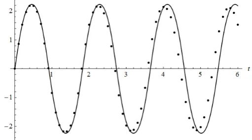
The 4th-order and 5th-order numeric solutions on the interval [0,6] with h = 0.1 are plotted in Figures 3 and 4, respectively. The 9th-order numeric solutions on the interval [0,10] with h=0.2 are plotted in Figure 5. We observe that the higher-order numeric solutions permit a larger step-size, and enlarge the effective region.

Figure 2. The exact solution *

( )

u t (solid line), the 5-term approximation φ5(t 0 0 9 ), , , (dot line), the 10-term appro-

ximation φ10(t 0 0 9 ), , , (dash line) and the 20-term approximation φ20(t 0 0 9 ), , , (dot-dash line).

[image:6.595.213.414.77.201.2]

Figure 4. The exact solution (solid line) and the 5th-order numeric solution on [0,6] with h = 0.1 (dots).

Figure 5. The exact solution (solid line) and the 9th-order numeric solution on [0,10] with h = 0.2 (dots).

3. Conclusions

We have developed higher-order numeric solutions for nonlinear differential equations based on the Rach- Adomian-Meyers modified decomposition method. Due to the new, efficient algorithms of the Adomian poly-nomials, the one-step numeric algorithm has a high efficiency, and permits us to easily generate a higher-order numeric scheme such as a 10th-order scheme, while for the Runge-Kutta method, there is no general procedure to generate higher-order numeric solutions. We demonstrated the presented numeric method by two nonlinear physical models.

Acknowledgements

This work was supported by the NNSF of China (11201308) and the Innovation Program of Shanghai Municipal Education Commission (14ZZ161).

REFERENCES

[1] G. Adomian, “Nonlinear Stochastic Operator Equations,” Academic, Orlando, 1986.

[2] G. Adomian, “Solving Frontier Problems of Physics: The Decomposition Method,” Kluwer Academic, Dordrecht, 1994.

[3] G. Adomian and R. Rach, “Inversion of Nonlinear Stochastic Operators,” Journal of Mathematical Analysis and Applications, Vol. 91, 1983, pp. 39-46.

[4] A. M. Wazwaz, “Partial Differential Equations and Solitary Waves Theory,” Higher Education and Springer, Beijing and Ber-

lin, 2009.

[5] R. Rach, “A New Definition of the Adomian Polynomials,” Kybernetes, Vol. 37, 2008, pp. 910-955.

[6] R. Rach, “A Convenient Computational Form for the Adomian Polynomials,” Journal of Mathematical Analysis and

Applica-tions, Vol. 102, 1984, pp. 415-419.

[7] A. M. Wazwaz, “A New Algorithm for Calculating Adomian Polynomials for Nonlinear Operators,” Applied Mathematics and

[image:6.595.202.427.237.357.2]

[8] J. S. Duan, “Recurrence Triangle for Adomian Polynomials,” Applied Mathematics and Computation, Vol. 216, 2010, pp.

1235-1241

[9] J. S. Duan, “An Efficient Algorithm for the Multivariable Adomian Polynomials,” Applied Mathematics and Computation, Vol.

217, 2010, pp. 2456-2467

[10] J. S. Duan, “Convenient Analytic Recurrence Algorithms for the Adomian Polynomials,” Applied Mathematics and Computa-

tion, Vol. 217, 2011, pp. 6337-6348

[11] R. Rach, G. Adomian and R. E. Meyers, “A modified Decomposition,” Computers & Mathematics with Applications, Vol. 23, 1992, pp. 17-23.

[12] G. Adomian and R. Rach, “Transformation of Series,” Applied Mathematics Letters, Vol. 4, 1991, pp. 69-71.

[13] G. Adomian and R. Rach, “Nonlinear Transformation of Series—Part II,” Computers & Mathematics with Applications, Vol. 23, 1992, pp. 79-83.

[14] G. Adomian and R. Rach, “Modified Decomposition Solution of Linear and Nonlinear Boundary-Value Problems,” Founda-

tions of Physics Letters, Vol. 23, 1994, pp. 615-619.

[15] G. Adomian, R. Rach and N. T. Shawagfeh, “On the Analytic Solution of the Lane-Emden Equation,” Foundations of Physics

Letters, Vol. 8, 1995, pp. 161-181.

[16] J. C. Hsu, H. Y. Lai and C. K. Chen, “An Innovative Eigenvalue Problem Solver for Free Vibration of Uniform Timoshenko Beams by Using the Adomian Modified Decomposition Method,” Journal of Sound Vibration, Vol. 325, 2009, pp. 451-470.

[17] G. Adomian, R. C. Rach and R. E. Meyers, “Numerical Integration, Analytic Continuation, and Decomposition,” Applied Ma-