LANCASTER UNIVERSITY
Model Predictive Control Structures
the Non-Minimal State Space
by
Vasileios Exadaktylos
This thesis is submitted in partial fulfilment
of the requirements for the degree of
Doctor of Philosophy
All rights reserved INFORMATION TO ALL USERS
The qu ality of this repro d u ctio n is d e p e n d e n t upon the q u ality of the copy subm itted. In the unlikely e v e n t that the a u th o r did not send a c o m p le te m anuscript and there are missing pages, these will be note d . Also, if m aterial had to be rem oved,
a n o te will in d ica te the deletion.
uest
ProQuest 11003427
Published by ProQuest LLC(2018). C op yrig ht of the Dissertation is held by the Author. All rights reserved.
This work is protected against unauthorized copying under Title 17, United States C o d e M icroform Edition © ProQuest LLC.
ProQuest LLC.
789 East Eisenhower Parkway P.O. Box 1346
This thesis is concerned with constraint handling for systems described by a N on- Minimal State Space (NMSS) form. Such NMSS models are formulated directly from the measured input and output signals of the controlled process, without resort to the design and im plementation of an observer. The thesis largely focuses on the application of Model Predictive Control (MPC) methods, a very common technique for dealing with system constraints. It is m otivated by earlier research into both NMSS and MPC systems, with features of both combined in this thesis to yield improved control.
The main contribution lies in the development of new m ethods for constraint handling of NM SS/M PC systems th a t contrasts with the ad hoc approach previ ously used for NMSS design based on the P roportional-Integral-P lus (PIP) algo rithm . S tructural aspects of NM SS/M PC design are considered, th a t result from m athem atical m anipulation of the closed-loop block diagram or from the definition of the state space description. The properties of these structures are investigated to provide an insight on features of the proposed strategies.
designer with additional freedom when using this tuning method.
There are many people to whom I am indebted for their support and friendship during my time in Lancaster.
F irst I would like to thank my supervisor Dr. C. James Taylor for his guidance and support during my PhD studies. He has been very helpful in scientific, for mality and personal m atters, and the results presented in this thesis are a result of useful conversations with him. Thanks also goes to Prof. Peter Young, Dr. Arun Chotai and Dr. Liuping Wang for fruitful conversations on control and NMSS issues.
Next, I would like to thank all the people th a t supported me throughout the years I spent in Lancaster; too many to mention w ithout forgetting many. Among them, special thanks goes to Kostas, Yannis and Eleni, whose friendship I shall always cherish.
I will always be grateful for the support th a t the General Michael Arnaoutis foundation and especially Mrs. Nathene A rnaouti has provided, both financially and personally. The Peel Trust is also acknowledged for financial support and the Faculty of Science and Technology for financially supporting my participation to the UKACC Control Conference 2006 in Glasgow.
D e cla r a tio n
I declare th a t this thesis consists of original work undertaken solely by myself at Lancaster University between 2004 and 2007 and th a t where work by other authors is referred to, it has been properly referenced.
C on ten ts
A b str a c t i
A ck n o w led g em en ts iii
D ecla ra tio n iv
C o n ten ts v
L ist O f T ables x
L ist O f F igu res xi
1 In tr o d u ctio n 1
1.1 M o tiv a tio n ... 1
1.2 NMSS and P roportional-Integral-Plus C o n tro l... 2
1.3 Model Predictive C o n tro l... 4
1.4 Academic C o n trib u tio n ... 5
1.5 Thesis O u tlin e ... 6
2 B ack grou n d C on cep ts 8 2.1 System id e n tific a tio n ... 9
2.2 O ptim isation te c h n iq u e s ... 10
2.2.1 The general constrained optimisation p r o b l e m ... 11
2.2.2 The MPC optimisation p r o b le m ... 14
2.2.3 Active set m e th o d s ... 15
2.2.4 Interior point m e t h o d s ... 16
2.3 Receding Horizon Control ( R H C ) ... 18
2.4 Lyapounov th e o r y ... 20
2.5 C o n c lu s io n s ... 22
3 R eferen ce governor over P IP con trol 23 3.1 System description and closed loop c o n t r o l ... 25
3.2 Control D e sc rip tio n ... 27
3.3 Stability and Reference Tracking ... 32
3.4 Simulation e x a m p le ... 32
3.5 Concluding re m a rk s ... 37
4 M P C w ith an in tegral—of—error s ta te 39 4.1 The controller of Wang and Young (2006) 40 4.1.1 System D e s c rip tio n ... 41
4.1.2 Control D escrip tio n ... 42
4.2 The alternative NM SS/M PC c o n tro lle r ... 44
4.3 Properties of the control s c h e m e ... 48
4.3.1 S et-point following and disturbance rejection ... 48
4.3.2 Stability a n a l y s i s ... 51
4.4 Simulation E x a m p le s ... 52
4.4.1 Double integrating p l a n t ... 52
4.4.2 The IFAC ’93 benchmark ... 54
4.5 C onclusion ... 58
5 M u lti-o b je c tiv e o p tim isa tio n 60 5.1 Predictive Control D e s c r ip tio n s ... 62
5.1.1 MPC with an integral-of-error state v a ria b le... 62
5.2 Tuning the M PC c o n tro lle r s ... 64
5.2.1 The goal attainm ent m e th o d ... 65
5.2.2 Application to M P C ... 66
5.3 Simulation E x a m p le s ... 67
5.3.1 SISO case: The IFAC ’93 b e n c h m a r k ... 68
5.3.2 MIMO case: The Shell Heavy Oil Fractionator Simulation . 72 5.3.2.1 Dynamic D e c o u p lin g ... 74
5.3.2.2 ‘Designed For’ R e s p o n s e ... 78
5.4 C o n c lu s io n s ... 82
6 T h e Forward P a th M P C 83 6.1 System and Control D e sc rip tio n ... 84
6.1.1 Stability a n a l y s i s ... 85
6.1.2 F e a s ib ility ... 86
6.2 Control s tru c tu re s ... 87
6.2.1 Feedback s t r u c t u r e ... 88
6.2.2 Forward p ath f o r m ... 89
6.2.3 C o n s tr a i n ts ... 91
6.3 Performance t e s t s ... 91
6.3.1 Monte Carlo Simulation (MCS) based uncertainty analysis . 92 6.3.2 Marginally stable s y s te m ... 94
6.3.3 The IFAC ’93 B e n c h m a r k ... 97
6.3.4 The ALSTOM B e n c h m a rk ...100
6.4 C o n c lu sio n s ... 107
7 D istu rb a n ce H an d lin g 109 7.1 In tro d u c tio n ...109
7.2.2 Direct use of the disturbance m o d e l... 113
7.3 Control D e sc rip tio n ...115
7.4 Simulation E x a m p le s ... 118
7.4.1 SISO E x am p le...119
7.4.1.1 Augmenting the state v e c to r... 120
7.4.1.2 Direct use of the disturbance m o d e l...120
7.4.1.3 Control S im u la tio n ...120
7.4.2 Control of a tem perature control in s ta lla tio n ...122
7.4.2.1 Description of the in s ta lla tio n ...123
7.4.2.2 System Id en tificatio n ... 125
7.4.2.3 Control and simulation re s u lts ...126
7.5 C onclusion...129
8 M P C for S ta te D ep en d e n t P ara m eter M o d els 132 8.1 In tro d u c tio n ... 132
8.2 The Reference Governor a p p ro a c h ... 134
8.3 M PC with an explicit integral-of-error state ...136
8.3.1 The basic algorithm ... 136
8.3.2 Improving the p r e d ic tio n s ... 137
8.3.3 Stability a n a l y s i s ... 140
8.4 M PC Formulation using an increment in the control a c t i o n ... 142
8.4.1 The basic algorithm ... 142
8.4.2 Improving the p r e d ic tio n s ... 145
8.4.3 Stability a n a l y s i s ...146
8.5 Simulation E x a m p le s ...147
8.5.1 S D P /P IP control and Reference M a n a g e m e n t... 147
8.5.2 S D P/M PC c o n t r o l ... 149
9 C o n clu sio n 156
9.1 Summary of r e s u l t s ... 156
9.1.1 Constraint handling with supervisory c o n tro l...156
9.1.2 The im portance of s t r u c t u r e ... 157
9.1.3 Timing of MPC c o n tro lle rs... 158
9.1.4 NM SS/M PC control of Non-linear s y s te m s ... 159
9.2 Directions for future research ...160
9.2.1 Control s t r u c t u r e ... 160
9.2.2 S D P/M PC c o n t r o l ...160
9.2.3 NM SS/M PC control a p p lic a tio n s ... 161
A p p e n d ic es 163 A N o ta tio n 164 A .l A c r o n y m s ... 164
A.2 N o m e n c la tu re ... 165
B C on vex sets and fu n ctio n s 167 B .l Convex S e t s ...167
B.2 Convex F u n c tio n s ... 168
C S ta b ility an alysis 171 C .l O ptim isation problem ... 171
C.2 Lyapounov s ta b ility ...172
List o f Tables
4.1 Param eter variations for the IFAC ’93 B e n c h m a rk ... 57
5.1 Param eters of the Shell Heavy Oil Fraetionator s im u l a t i o n ... 72 5.2 Integral of absolute error values for three control structures after
m ulti-objective optimisation of their param eters . ... 31
6.1 Bounds of param eter uncertainty th a t results in the stochastic closed loop poles lying within 0.1 of the nominal case for the IFAC ’93 Benchmark ... 98 6.2 Boundary values for the control signals of the ALSTOM nonlinear
gasifier system ... 103 6.3 Integral of absolute error values for the ALSTOM nonlinear gasifier
s y s t e m ... 105
7.1 Dimensions of the matrices in the state space form ... 112 7.2 Sum of absolute errors for the two control structrues th a t accound
for the disturbance model and two that do not ...123 7.3 Input, O utput and D isturbance s i g n a l s ... 125 7.4 Input and rate-of-change b o u n d s ... 127
List o f F igures
2.1 The Receding Horizon Control s tr a t e g y ... 20
3.1 The Reference Governor Control S c h e m e ... 24 3.2 Unconstrained closed loop response of a marginally stable non
-minimum phase s y s te m ... 34 3.3 Constrained closed loop response of a marginally stable non-m inim um
phase system with and w ithout a Reference G o v e r n o r... 35 3.4 Comparison of RG systems with different prediction horizons . . . . 36 3.5 The (3 RG param eters for different prediction horizons ... 37
4.1 Block diagram of the M PC control scheme based on a model de scription with an integral-of-error state v a r ia b le ... 50 4.2 Presentation of the disturbance rejection properties w ith a closed
loop simulation of the double integrating p l a n t ... 54 4.3 Nominal response for the IFAC ’93 benchm ark of the M PC con
troller based on a model with an integral-of-error state variable . . 56 4.4 Robustness test for the IFAC ’93 benchmark of the M PC controller
based on a model with an integral-of-error state v a r ia b le ... 56 4.5 Robustness test for the IFAC ’93 benchmark of the NM SS/M PC
controller of Wang and Young ( 2 0 0 6 ) ... 57
5.1 Presentation of the multi-objective performance optim isation tech nique for IFAC 93 simulation for the controller based on a system with an explicit integral-of-error state v aria b le... 69 5.2 IFAC 93 simulation before and after multi-objective optim isation
for the controller of Wang and Young ( 2 0 0 6 ) ... 71 5.3 Decoupling of the Shell Heavy Oil fractionator example for the
NMSS controller of Chapter 4 ... 75 5.4 Decoupling of the Shell Heavy Oil fractionator example for the
NMSS controller of Wang and Young ( 2 0 0 6 ) ... 77 5.5 ‘Designed for’ response of the Shell Heavy Oil fractionator example
for three control s tr u c tu re s ... 79
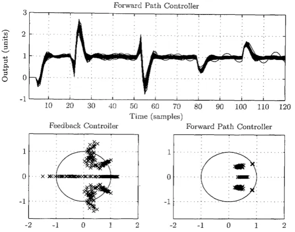
6.1 NM SS/M PC represented in feedback form... 89 6.2 NM SS/M PC represented in forward p ath form ... 90 6.3 Pole positions for param eter variation in the num erator param eters
for the Forward P ath and the Feedback MPC c o n t r o l le r s ... 94 6.4 Pole positions for param eter variation in the denom inator param e
ters for the Forward P ath and the Feedback M PC controllers . . . . 95 6.5 Pole positions and system output for param eter variation in the
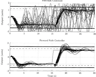
denom inator param eters for the Forward P ath and the Feedback M PC co ntrollers... 96 6.6 Closed-loop simulations of the IFAC ’93 benchmark with the para
metric variation at Stress Level 2 for the Feedback and the Forward P ath c o n tro lle rs ... 99 6.7 Closed loop simulations of the IFAC ’93 benchm ark with the para
metric variation at Stress Level 2 for the Forward P ath controller after m ulti-objective optimisation of the weighting param eters . . . 101 6.8 System outputs of the ALSTOM gasifier in response to a pressure
6.9 System inputs of the ALSTOM gasifier in response to a pressure sine wave disturbance at 100% load using the forward path form. . 104 6.10 R ate-of-change for the four control input signals of the ALSTOM
gasifier system at 100% load using the feedback form ... 105 6.11 R ate-of-change for the four control input signals of the ALSTOM
gasifier at 100% load using the forward p ath form... 106
7.1 System output for disturbance rejection for structures th a t account for the disturbance model ... 121 7.2 System output for disturbance rejection for structures th a t do not
account for the disturbance m o d e l... 122 7.3 Schematic of a tem perature control installation ... 123 7.4 Step experiment for estimation purposes of the tem perature control
installation ... 125 7.5 Estim ated and actual output d ata for the tem perature control in
stallation ...127 7.6 Result of the control simulation example for the tem perature control
installation ... 128 7.7 System Inputs for the control simulation of the tem perature control
installation ... 129 7.8 Mean and Maximum absolute error for the control simulation of the
tem perature control in s ta lla tio n ... 130 7.9 The rate-of-change of the inlet tem perature for the controller th a t
takes into account the disturbance model and the one th a t does not 130
8.1 Response of the closed loop S D P /P IP control system w ithout con strain ts... 149 8.2 Comparison of the S D P /P IP scheme with and w ithout R G ... 150 8.3 Closed loop response for the SD P/M PC control scheme based on a
8.4 The value of the cost function for the S D P /M P C controller with an explicit integral-of-error s t a t e ...151 8.5 Closed loop simulation for the S D P /M P C controller w ith an incre
ment in the control action... 152 8.6 O utput prediction trail for the SD P /M P C controllers w ith and w ith
out the improvement in the p re d ic tio n s ... 153 8.7 The value of the cost function for the S D P /M P C controller with an
C hap ter 1
In tro d u ctio n
1.1
M o tiv a tio n
Every physical system is subject to constraints. A car for example has a maximum acceleration (th at depends on the loading of the car, the terrain it drives on, etc.) and a maximum speed (again dependent on various factors). Furthermore, safety issues impose additional constraints, such as an upper speed limit when cornering or when travelling in an urban area. The above rather simple everyday example makes apparent the need to account for various constraints when dealing with any kind of physical system.
need to operate very close to or on the limits of constraints for an acceptable performance to be achieved.
Research th a t has previously been conducted at Lancaster University on control systems, has focused on systems described by a Non-M inimal State Space (NMSS) form and has revealed some interesting properties of such systems (see Section 1.2 for a brief description). However, there was no inherent consideration for system constraints when dealing with systems described in such a way until recently when Wang and Young (2006) proposed a Model Predictive Controller (MPC) based on a NMSS system description. In the same direction, this thesis exploits the structural properties of this controller and considers the properties of various other N M SS/M PC control systems proposed by the author. More specifically, systematic approaches of constraint handling when dealing with NMSS systems are sought by combining results from both NMSS and MPC fields.
1.2
N M S S and P r o p o rtio n a l—In teg ra l—P lu s C on
tro l
roportional-Integral-Derivative (PID) controller.
Since then, a lot of theoretical contributions have been presented th a t develop and extend the N M SS/PIP control scheme. For example, Wang and Young (1988) further extended the P IP control theory; structural aspects of N M SS/PIP control have been considered by Taylor et al. (1996); Young et al. (1998) and Chotai et al. (1998) developed the P IP controller for continuous time systems described in an NMSS form; Taylor et al. (1998) evaluated a Smith Predictor to account for pure tim e delays in the system; while Taylor et al. (2000a) revealed the relationship between P IP and the Generalised Predictive Controller (GPC) of Clarke et al. (1987a, b).
In addition to the theoretical results, the N M SS/PIP controller has been tested in a wide range of real applications. For example, Taylor et al. (2000b) applied P IP control to a carbon dioxide enrichment process; Q uanten et al. (2003) used P IP for tem perature control within a car; Gu et al. (2004) used the P IP controller for an autonomous excavator; Taylor et al. (2004b) designed a P IP controller for ventilation of agricultural buildings; Van Brecht et al. (2005) controlled the 3-D distribution of air within a ventilation chamber; and Taylor et al. (2006b) applied the P IP controller to the very demanding application of a vibro-lance.
1.3
M o d e l P r e d ic tiv e C on trol
Model Predictive Control (MPC) is a widely used technique, especially in the chemical and process control industries (Qin and Badgwell, 1996). According to M orari (1994) MPC dates back to the 1960s, while the paper by Kwon and Pearson (1977) establishes the foundations for MPC in a form similar to the one used today. A further great step in the evolution of M PC is the Generalised Predictive Controller (GPC) of Clarke et al. (1987a,b) th a t initiated a whole new area of research. More recently Bemporad et al. (2002) have exploited the state feedback structure of MPC and introduced an explicit solution th a t makes the on-line solution of an optimisation obsolete. In this latter work, the authors divide the state space into smaller areas where a feedback controller th a t satisfies the constraints can be calculated. Depending on the state of the system, the appropriate feedback controller needs to be chosen degrading the optimisation problem to one of finding the appropriate feedback controller from a look-up table.
During the last decades, a lot of researchers have been working on different areas of M PC such as it’s stability (for example Mayne and Michalska, 1990; Rawlings and Muske, 1993: Bemporad, 1998b; Primbs and Nevistic, 2000; Bloemen et al., 2002; Cheng and Krogh, 2001, present stability results for various M PC problem formulations) or it’s optimality (e.g. Scokaert et ah, 1999; Kouvaritakis et al., 2000, consider sub-optim al solutions to the MPC problem). A comprehensive review of stability and optimality of MPC is performed by Mayne et al. (2000). Various robust solutions have been presented (some approaches include those of K othare et al., 1996; Badgwell, 1997; Magni, 2002; Fukushima and Bitmead, 2005), while a review is made by Bemporad and Morari (1999). Finally, a lot of effort has been put in reducing the on-line com putational load (see for example Borrelli et ah, 2001; Kouvaritakis et ah, 2002; Bacic et ah, 2003; Grieder et ah, 2004; Imsland et ah, 2005, and references therein).
Young (2006) th a t presented a MPC scheme using a NMSS framework (another NMSS approach to M PC can be found in Chisci and Mosca, 1994) th a t led to improved results compared to existing structures using a minimal state space de scription. Variations of the NM SS/M PC structure are considered and the NMSS system description is exploited to allow for improved simulation results when com pared to existing m inimal representations of MPC.
1.4
A ca d em ic C o n trib u tio n
As already stated, the main topic of this thesis is to incorporate system atic con straint handling techniques into the NMSS framework extending the work of Wang and Young (2006); and to use experience and methodology developed for the PIP controller to the proposed M PC/NM SS control structures.
More specifically research carried out has contributed towards:
• The importance of structure in the N M SS/M P C control scheme. Various
predictive structures are presented throughout the main body of this thesis. By exploiting the properties of NMSS models and considering approaches evaluated for P IP control, different model descriptions are considered (Chap ters 3, 4 and 7), their properties are presented and comparisons among them are made. Furthermore, an alternative N M SS/M PC control structure th a t makes use of an internal model is considered (namely the Forward P ath Controller, Chapter 6); i t ’s properties are presented and it ’s performance is compared to conventional NM SS/M PC in the presence of model uncertainty.
• Tuning of M PC Controllers. An autom atic tuning technique is presented
M PC control structures is compared and it is shown th a t the NM SS/M PC controller introduced in Chapter 4 forms the structure of choice when using this tuning technique.
• M P C of State Dependent Parameter (SDP) models. C hapter 8 of the thesis
considers constraint handling for the potentially highly non-linear class of SDP models. This is the first approach in this direction and can lead to better understanding of control of such systems. An iterative algorithm is proposed th a t utilises the predicted output to form a prediction of the system matrices. The predicted system evolution is subsequently used to form a new predicted output th a t is closer to the actual o utput of the system (based on the calculated control trajectory). In contrast to existing approaches of MPC of non-linear systems a simple stabilising algorithm is presented th a t is based on improved predictions and assumptions very similar to the linear case.
1.5
T h esis O u tlin e
The rest of the thesis is organised as follows. C hapter 2 provides some neces sary background m athem atical concepts on system identification and optimisation. Furtherm ore, the notions of Receding Horizon Control (RHC) and Lyapounov sta bility th a t are used throughout the rest of the thesis are briefly reviewed.
C hapter 3 presents a reference management technique and focuses on applica tion to existing PIP-controlled systems. Via simulation examples it is shown th a t a Reference Governor (RG) can provide a fast and reliable solution to constraint handling in existing control applications.
tives providing the necessary framework for trade-off between the objectives. It is furtherm ore shown th a t the control structure presented in C hapter 4 provides a more flexible framework compared to existing M PC realisations when using this tuning method.
Next, C hapter 6 evaluates experience from P IP control and alters the structure of the controller of Wang and Young (2006) and proposes a potentially more robust NM SS/M PC control structure, namely the Forward P ath controller.
Chapter 7 considers NM SS/M PC control in the presence of modelled measured disturbances. Two structures are considered th a t lead to improved closed loop response when compared to the conventional NM SS/M PC approach th a t does not account for the disturbance model. Furthermore, a case study of an actual tem perature control ventilation installation is presented and one of the proposed structures is simulated for this particular application.
C hapter 8 deals with the constraint handling problem for the highly non-linear class of SDP models. The RG approach of Chapter 3 is initially considered, while a direct application of MPC is described later in the same chapter. The evolution of the system matrices is subsequently considered to improve the state and output predictions leading to two NM SS/M PC controllers w ith guaranteed asymptotic stability under assumptions very similar to the case of linear systems.
C hap ter 2
B ackground C on cep ts
This chapter introduces some concepts th a t are present in M PC systems. It pro vides the necessary background on issues th a t arise by presenting existing results and methods. Moreover, references are given to more advanced and detailed text books in each subject. However, since it is intended to be a reference chapter, formal proofs are om itted and only the essence of some ideas is highlighted.
Initially some background information on system identification techniques is given in Section 2.1. The general discrete-tim e difference equation th a t is used throughout the thesis is given and methods to identify it from open-loop simulation d a ta are highlighted. Furthermore an introduction to estimation of the system uncertainty is given, th a t is used in some of the simulations in chapters th a t follow (in Section 6.3.2 for example).
The MPC law is derived by the minimisation of a cost function subject to constraints. Therefore, some key concepts of constrained optim isation theory are provided (Section 2.2). Additionally, a brief presentation of Receding Horizon Control (RHC), which is the key concept to applications of M PC is made (Sec tion 2.3). Although RHC is a well understood technique, some of i t ’s basic ideas are still presented and discussed for completeness.
ity, the widely used Lyapounov theory can be employed. The basic conclusions of Lyapounov stability theory for discrete-tim e systems are therefore presented in Section 2.4 and reference to them is made in the main body of the thesis (e.g. in Sections 4.3.2 and 6.1.1 where the stability of different control structures is con sidered).
2.1
S y ste m id en tifica tio n
In order to develop a control algorithm, a linearised representation of the system is first required. For non-linear systems, the essential small perturbation behaviour can usually be approximated well by simple linearised transfer function models. Although different model structures have different properties in control system design (see Pearson, 2003, for a review of non-linear models in control), the present thesis considers only the following linear, g-input, p -o u tp u t discrete-tim e system, w ritten in difference equation form as follows,
Yk + A-iYk-i + . .. + A ny k_n = B iU ^-i + B 2Ufc_2 + . . . + B mUfc_m (2.1)
where the subscript k is a sampling index (i.e. yk = y{k))\ y = [yi y2 • • • yP]T
and u = [u\ u 2 . .. uq]T are the vectors of output and input variables respectively; while Ai, i = 1,2, ...,n and B i; i = 1,2, ...,ra are p x p and p x q matrices of system coefficients.
algorithms (Young, 1976, 1984, 1991), since these are optim al in statistical terms and often more robust to noise model specification th an alternative estim ation pro cedures (Young, 2006). Such statistical estimation analysis results in an estimate p of the reduced order param eter vector p and an associated covariance m atrix P*. For transfer function models, the standard errors on the param eter estimates are then com puted directly from the square root of the diagonal elements of P*. Also, P* provides an estimate of the uncertainty associated with the model param eters, which can be employed in Monte Carlo analysis to investigate the robustness of various control designs.
Finally, for a given physical system, an appropriate model structure first needs to be identified, i.e. the order of the various polynomials and the pure time delays in sampling intervals. In the latter regard, it is straightforward to introduce into equation (2.1) a time delay between the control signal and the ou tput by assuming th a t the appropriate coefficients in B* are zero. The two main statistical measures employed to help determine the model structure are the coefficient of determ ination based on the response error, which is a simple measure of model fit; and the Young Identification Criterion (YIC), which provides a combined measure of fit and param etric efficiency, with large negative values indicating a model which explains the output d ata well, w ithout over-param etrisation (Young, 1991).
2.2
O p tim isa tio n tech n iq u es
This section provides some background concepts on optim isation and the related m athem atical notions. For brevity and simplicity, formal proofs of theorems are om itted, b ut reference is made to publications in which they can be found. At this point it should be noted th a t optimisation is a huge area of ongoing research and a great number of publications exist. However, this is ju st a simple presentation of some results th a t are used specifically in MPC.
numerous researchers and different research groups around the world (e.g. Biegler, 1998; Borrelli et ah, 2001; Chisci and Zappa, 1999; Diehl and Bjornberg, 2004; Rao et ah, 1998) th a t is not covered here. Moreover, specific attention should be paid on explicit solutions to the MPC problem (e.g. Bemporad et ah, 2002; Grieder et ah, 2004; Rossiter and Grieder, 2005) th a t make the online optim isation obsolete. However, this is out of the scope of this thesis and such m ethods are not presented here.
In the following, mention is made to convexity of sets and functions th a t is im portant in constrained optimisation (and is the same as the M PC problem con sidered throughout the thesis). Definitions and basic theorems related to convexity are presented in Appendix B.
2.2.1
T h e g e n e ra l c o n s tra in e d o p tim is a tio n p ro b le m
The general form of a constrained optimisation problem can be described as follows:
The next theorem gives the conditions under which local and global minima for the problem (2.2) coincide, along with a condition for the uniqueness of a solution.
T h e o r e m 2.2.1 (Global and unique minima (Goodwin et ah, 2005)). Consider' the
problem defined in (2.2), where X is a nonempty convex set in and f : X —> 9ft
is convex on X . I f x* 6 X is a local optimal solution to the problem, then x* is a
global optimal solution. Furthermore, if either x* is a strict local m inimum, or if
f is strictly convex, then x* is the unique global optimal solution.
minimise /( x )
subject to: gfix) < 0 i = 1, 2 ,. . . , m h j(x) = 0 j = l , 2 , . . . , l
x G X
Next, the K arush-K uhn-Tncker (KKT) necessary and sufficient conditions are presented. They provide the necessary and sufficient conditions under which a feasible1 solution of the problem (2.2) is a local or global minimum. Combining them with Theorem 2.2.1, the conditions for a feasible solution of (2.2) to be a unique global minimum can be derived. Furthermore, the K KT conditions are employed by algorithms th a t solve the problem (2.2) such as the ones presented in Sections 2.2.3 and 2.2.4.
T h e o r e m 2 .2.2 (K arush-K uhn-Tucker Necessary Conditions (Goodwin et ah, 2005)). Let X be a nonempty open set in 3?n; and let f : ffi1 —> gi : —» 3^
and hj : 5?n —>• 5? for i = 1, 2 , . . . , m and j = 1 , 2 , . . . , / . Consider the problem
defined in (2.2). Let x be a feasible solution, and X — {i \ gi{x) = 0}. Suppose
that f and gi, fo r i G I are differentiable at x , that each gi; fo r i X is con
tinuous at x., and that each h,j fo r j = 1 , 2 , . . . , / is continuously differentiable at
x.
Furthermore, suppose that V ^ ( x ) r and V /q(x)T fo r i G X and j = 1, 2, . . . , /
are linearly independent. I f x is a local optimal solution, then there exist unique
scalars Xg. and A^ . fo r i G X and j = 1, 2 , . . . , /; such that: i
V /(x)r
+ Y A 9lV gi(x )T + Y i \ V h j ( 5 i f = 0i£Z j=1
A g{> 0 i G X
Furthermore, if gi, i ^ X are also differentiable a t x , then the above conditions can
be written as:
m I
V /(x)T +
Y
K V3i(x)T
+
Y
^ Vft3-(x f = 0
i=1 j=1
A3i5'(x) = 0 i = l , 2 , . . . , m
Xgi > 0 2 — 1 , 2 , . . . , 771
T h e o r e m 2.2.3 (K arush-K uhn-Tucker Sufficient Conditions (Goodwin et ah, 2005)). Let X be a nonempty open set in $Rn; and let f : gi : $Rn —> -ft
and hj : 5Rn —■> 5ft for' i = 1, 2 , . . . . m and j = 1, 2, . . . ,1. Consider the problem
defined in (2.2). Let
x
be a feasible solution, and X — {i : gi(x) = 0}. Supposethere exist scalars X*. and \*hj for i G X and j = 1, 2, . . . ,1, such that
i
V / ( x ) r + ] T A ; v 3,(x )r + V /V /^ ( x ) r = o (2.3)
i£l j=1
Let J = j j : \*h. > o j and K, = |jf : X*x. < o | . Further, suppose that f is
pseu-doconvex at x , gi is quasiconvex at x fo r i G X, hj is quasiconvex at x fo r j G J ,
and hj is quasiconcave (i.e. —hj is quasiconvex) at x fo r j G 1C. Then x is a global
optimal solution to problem (2.2).
Although the form (2.2) is convenient to extract valuable results for the opti misation problem, in the MPC framework it is usually formed in a way where the constraints are presented in a more compact m atrix form as is shown for example in the next section (Equations (2.4b) and (2.4c)). In this regard, it would be more convenient to write the KKT conditions in a compact m atrix form as follows:
V /( x ) r + V g ( x ) TAj + ' V h ( x ) TXj = 0
>h9 (x) = 0
Aj > 0
where V g (x ) is the m x n Jacobian m atrix whose zth row is V<ft(x); V k ( x ) is the I x n Jacobian m atrix whose ith row is V /p(x); g (x ) is a vector whose zth element is <ft(x); and A* and Aj are vectors containing the Lagrange multipliers A» and Xj respectively.
creasing w ithout violating the imposed constraints. In other words, the derivative of the cost function can be described by a linear combination of the derivatives of the constraint regions at the minimising point. An interesting geometrical inter pretation of the KKT conditions can be found in Papalambros and Wilde (2000).
A lthough the cost function in MPC can be of any kind, it is very common for a quadratic cost function to be minimised subject to equality and inequality con straints, while an interesting consideration of the results of using a linear cost function can be found in Rao and Rawlings (2000). The general problem for m ulation with a quadratic cost function th a t is used in the rest of the thesis is:
where, A e and A j are matrices th a t represent the equality and inequality con straints and the inequality sign refers to element by element inequalities.
Prom Lemmas B.1.4 and B.2.3 it follows th a t the optim isation problem defined above is one of minimising a convex function over a convex set and according to Theorem 2.2.1 any local minimiser is a global one. Furtherm ore if H >- 0, i.e. H is positive definite, then from Theorem 2.2.1 it results th a t this global minimiser is unique.
It follows th a t a necessary and sufficient condition for a point x* to be a unique global minimiser of (2.4) is for the KKT conditions to be satisfied, i.e. there exist Lagrange multipliers A; for i e l — {i,A j x < 0} and A j for j e £ = {i,A E5t = 0}
2.2.2
T h e M P C o p tim is a tio n p ro b le m
minimise { x TH x + p Tx } subject to: A ^ x = 0
A / x < 0
such that:
H x + p r -j- A/A; + A^Aj = 0 (2.5a)
Aj > 0 (2.5b)
X j ( A j x — b/) = 0 (2.5c)
where, A i and A j are vectors containing A * and Xj respectively. It should be noted here th a t (2.5c) is added to account for the inactive inequality constraints (for more details see Goodwin et ah, 2005). Furthermore, it is clear th a t the inequality and equality constraints of (2.4) must also be satisfied at x*.
This section introduced the quadratic program th a t will be used throughout this thesis and presented the KKT conditions for it. It is evident th a t it takes a simpler form than the general one and as mentioned before, a lot of efficient algorithms exist to solve this simplified problem. The underlying ideas of the two most commonly used categories of algorithms are presented in the next two sections.
2.2.3
A ctiv e se t m e th o d s
In active set methods, it is assumed th a t an initial feasible solution exists (although this is a difficult problem on its own, especially in large optimisation problems). At this point the active constraints are identified and a decreasing direction d is sought such th a t / ( x ) < / ( x fc), where x fc is the initial feasible solution and x = xj, + d. If x is feasible for the original problem (2.2), then it is set as an initial condition and the same procedure is repeated. If not, then a line search is made along the direction of d to identify the point were feasibility is lost (i.e. the point at which a previously inactive constraint becomes active). This procedure is repeated until there is no decreasing direction, i.e. d = 0.
as a global minimum and the algorithm stops. If not, then there is a direction along which some active constraint becomes inactive and the function
/(x)
has a smaller value. This constraint is identified by i t ’s associated Lagrange multiplier in the K KT conditions (it is negative). Then a descent direction away from this constraint is calculated and the algorithm proceeds on to the next iteration.More information on the details of active set methods can be found in Fletcher (1981) and Gill et al. (1981), while the above presentation is a summary of infor m ation found mainly in Maciejowski (2002) and Goodwin et al. (2005).
An attractive feature of active set methods is th a t the solution lies all the time inside the feasible region. So, in cases were the algorithm needs to be term inated before the global minimiser has been found, the solution would be feasible, which is very im portant in real applications (feasibility can be more im portant than optim ality in some cases (Maciejowski, 2002)). Yet, the problem of finding an initial feasible solution is hard enough for the general case (even with the quadratic program of (2.4)) and a drawback for active set methods. However, in the case of M PC, the previous solution to the problem can provide (in the absence of large disturbances) not only a feasible solution, but also one th a t is close to the optimal one.
An active set method is evaluated by the
quadprog
function (that is used in the simulations presented in this thesis) of the M ATLAB® optim isation toolbox in ‘M edium -Scale’ mode (i.e. in most cases considered in this thesis).2.2.4
In te rio r p o in t m e th o d s
th a t a lot of them don’t necessarily require a feasible initial point (making the problem easier to solve, although a good initial guess can drastically improve the convergence of the algorithm (Melman and Polyak, 1996)). However, the m ajority of them will not provide a feasible solution until the end of the optimisation pro cedure, which can cause problems in large scale problems where a feasible solution is required even if the algorithm has not term inated (as already mentioned in the description of the Active Set methods in Section 2.2.3).
In a bit more detail, the idea underlying the prim al-dual interior point methods is presented here. In this class of algorithms, a barrier' function is introduced th a t is dependent on the constraint region of the initial optim isation problem and the following unconstrained problem is introduced:
minimise
{/(x)
- fbarrier(v,^(x )>
hj i x ))} (2-6)where / barrier (') is a function th a t th a t monotonically decreases while fi —> oo; and /(•), gi(-), i = 1, . . . , m and hj(-), j = 1 , . . . , / are defined in (2.2). Both (2.6) and i t ’s dual are subsequently solved sequentially for increasing values of /i. It can be shown th a t as /i increases, the solutions of the primal and dual problems come closer and eventually converge to the solution of the initial constrained prob lem (2.2).
There are a lot of variations and algorithms for interior point methods in the literature. A collection of some, along with a discussion on some issues th a t arise can be found in Anstreicher and Freund (1996). Some intuitively nice guidelines are also given by Maciejowski (2002) and Goodwin et al. (2005), while Rao et al. (1998) present an optimisation algorithm th a t exposes the structure of the MPC problem for improved speed.
2.3
R ece d in g H orizon C on trol (R H C )
As already mentioned the control law to be applied to the system results from an optim isation problem th a t can take the form of (2.4). To introduce the notions of prediction and control horizon, the following optim isation problem is defined:
NP Nc- 1
minimise
E
X f c + i Q x f c + i "bE
(2.7a)i=1 i—0
subject to: x fc+i = / ( x fc+i_i, u fc+i_i) (2.7b) x fc+i G X i = 1 , . . . , Np (2.7c)
u k+i e U i = 0 , . . . , N c - 1 (2.7d)
where the minimisation is performed over the control input sequence {ufc+^fc},
% = 0 , . . . . N c — 1, where the subscript |k defines the sampling instant at which the prediction is based on and A and U represent constraint sets on the state and inputs of the system respectively. This is in the form of the well-known Linear Q uadratic Regulator (Mosca, 1995) with the addition of constraints, but instead of taking into account the system evolution x fc+i = / ( x fc+i_i, u k+i-i) for i = 1 , . . . , oo, only Np steps ahead are considered, and Np is called the prediction horizon. In the same manner N c future values of the control signal are sought, and N c is called the control horizon. Details on how to bring the problem (2.7) in the form of (2.4) are given in later chapters for the specific cost function th a t is used in each MPC formulation of the problem.
However, something unexpected can happen before the end of this horizon (when a new control sequence would be calculated). In this case the predicted system evolution differs from the actual one. To avoid this kind of mismatch, (2.7) is solved at every sampling instant and the receding horizon strategy is evaluated.
and the optim isation problem is solved again. In more detail, the control steps are described in the following.
1. At time instant k the problem (2.7) is solved and the optimal sequence { u fc|fc,. . . , Ufc+w.-ip} is calculated.
2. The first first value of the control sequence is applied to the system and the rest is discarded.
3. A new measurement of the system state x fc+1 is made at the following sam pling instant k + 1.
4. Based on the new measurement the optimisation problem (2.7) is solved again and a new control sequence { ufc+1|fc+i , . . . , u&+wc|ah-i} is calculated.
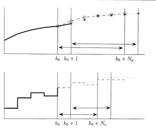
A graphical representation of the RHC strategy is given in Figure 2.1. The prediction and control horizons are shown, while it becomes apparent th a t they slide along to the future, at each sampling instant.
It is clear th a t in the disturbance free case and when there is no model mis match, the difference in the optimal control sequences reduces by increasing the control and prediction horizons and eventually it converges to the optimal solution of the infinite horizon control problem (in the absence of constraints).
Figure 2.1: The Receding Horizon Control strategy. It is evident th a t a mismatch between the predictions of two consecutive sampling instant may occur.
2.4
L yap ou n ov th eo ry
A very general definition of stability is the one of B ounded-Input B ounded-O utput stability as defined below.
D e fin itio n 2.4.1 (Boundecl-Input Bounded-O utput Stability (Marlin, 1995)). A system is stable if all output variables are bounded when all input variables are
bounded
However, the above definition is quite general and although it provides a useful insight on the notion of stability, it is not very helpful when it comes to formally addressing this issue. In this regard, the more widely used Lyapounov stability is considered below, according to which an equilibrium point is stable if a small perturbation of the state or input results in a continuous perturbation of the subsequent state and input trajectories. More formally, it is defined as:
D e fin itio n 2.4.2 (Lyapounov Stability (Letov, 1961)). Let S be a set in 3Rn that
[image:37.543.129.444.92.355.2]system
Xfc+i = / ( x fc, u fc) (2.8)
with Xfc G 5ftn, has an equilibrium point at (x, u), that is / ( x , u) = x. Let Xfc0 G <5
and {xfc0+,;} G 5 , fo r i > 1, 6e the resulting sequence satisfying (2.8) fo r a control
sequence Uk0+i, i > 1. The equilibrium point is stable in S if fo r any e > 0, there
exists 5(e) > 0 such that
XfcQ G S and
T (Xfco - x )T , (u ko - u )T || < 5
(xfco+i - x )T , (u ko+i - u ) T
T
< e, Vi > 0
T
Furthermore, if in addition || (xfc0+i — x) , (ukQ+i ~ u)
it is asymptotically stable.
0 as i —> oo then
Since it is the most widely used stability definition and has been extensively used in the literature, in the rest of the thesis only Lyapounov stability is con sidered. The notion of Lyapounov stability of an equilibrium point requires the system to remain near th a t point after a disturbance in the state or the input of the system, while asymptotic stability requires for the equilibrium point to be reached eventually. The most common way of showing th a t a point is Lyapounov stable in nonlinear control theory is by means of Lyapounov’s theorem th a t is presented below.
L y a p o u n o v ’s T h e o re m . (Maciejowski, 2002). If there is a function V (x ,u ) which is positive definite, with C (x ,u ) = 0 only if (x, u) = (0 ,0 ), and has the property th a t
II [xi,Ui] II > II [x2,U2] II => ^ ( x ^ U i ) > y ( x 2, u 2)
of (0, 0) the property
V(xk+Uuk+1) < V{xkluk)
holds, then (0,0) is a stable equilibrium point. If, in addition, V(xfc,u*.) —>• 0 as
k —> oo then it is asymptotically stable. Such a function is called a Lyapounov function
Lyapounov’s theorem states the conditions for stability and asym ptotic stabil ity of the origin. Yet, with a change in the system coordinates any equilibrium can be moved to the origin. Therefore, the Lyapounov theorem can be applied to prove stability of any equilibrium point.
A stability proof for the general MPC scheme can be found in Appendix C th a t poses the basis for stability proofs throughout this thesis.
2.5
C o n clu sion s
C hap ter 3
R eferen ce governor over P IP
con trol
As already mentioned, a common control structure for systems described in the NMSS is Proportional-Integral-Plus (PIP) control, th a t can be considered a pow erful extension of the well known Proportional-Integral-D erivative (PID) control scheme. In the cases however where constraint handling is an issue, P IP (and PID) control is designed off-line in an ad-hoc m anner to avoid constraint viola tion (e.g. Taylor et al., 2001; Taylor arid Shaban, 2006, adjust the LQ weights using off-line simulations).
Two common techniques to deal with constraint handling when a controller is already available are the Closed Loop Paradigm (CLP) (e.g. Rossiter, 2003) and the Reference Governor (RG) (e.g. Bemporad et al., 1997). In both, an optimal supervisory control scheme is applied to the already controlled system to ensure constraint satisfaction. Although it can be proved th a t both control schemes are equivalent (Rossiter, 2003) with the only difference being in the way the degrees of freedom (dof) are parametrised, they have different properties regarding the conditioning of the resulting optimisation problem and the insight they provide as to the effect of the constraints to the closed loop system.
This chapter considers the problem formulation as in th a t of the RG, while
Reference Output
Precompensated System
Controller System
Reference Governor
Figure 3.1: The Reference Governor Control Scheme
param etrising the dof as perturbations around the reference signal (even though this is more common in the CLP approach, it is chosen here due to i t ’s simplicity and the insight it can provide on the effect of the constraints on the closed loop system ). The underlying idea of RG techniques is th a t as long as a stable controller exists, there can be a reference sequence th a t can lead to constraint satisfaction whilst preserving the closed loop system properties for this artificial reference (or for the actual one when operating far form the constraints). It can also be considered as a nonlinear reference filter th a t alters the reference signal when it would cause constraint violation if it was directly applied to the system. A block diagram of the RG control scheme is presented in Figure 3.1.
The approach presented in this chapter is a first attem pt for systematic con straint handling within the NMSS. It can easily be applied to systems were a PIP controller is already available and improve the performance of the overall control scheme (as is shown by a simulation example in Section 3.4). The same technique is later evaluated for an initial approach to constraint handling in the more demand ing context of the non-linear class of State Dependent Param eter (SDP) models as described in Chapter 8. Reference will be made here for the basic notions of the RG scheme and formulation of the control problem.
and w ithout a RG. Finally, Section 3.5 concludes the present chapter.
3.1
S y ste m d escrip tio n and clo sed lo o p con trol
Consider the g-input p -o u tp u t system described by the difference equation (2.1). As described in Young et al. (1987), the system described by (2.1) can take the following NMSS form:
x fc = A x fc_i + B u fc_i + D r fc
Yk = C x fc
(3.1a) (3.1b)
where r = [r\ r 2 ■ • • rp]T is the reference level vector and the ( n + l) p + m ( g — 1) x 1 state vector x is defined as:
r T T T T T
X f c = [ y I y j f e - 1 • • • Y k - n+1 U fc- 1 u k -2 uk —m + 1 zTl k J (3.2)
in which = x-z~T (r/c — Yk) is the integral-of-error state variable th a t is used to ensure type one servomechanism performance (e.g. Taylor et ah, 2000a). The system matrices in (3.1) are:
A =
-A x •• A n_x A n b 2 • B m_x B m O p
I p •• O p O p 0 p q O p q O p g O p
oP • Ip O p 0 p q O p g O p g O p
0 q p 0 q p 0 q p 0 , •• ■ o9 0 g O g p
0 q p 0 q p O q p I, • o9 0 , O q p
0 q p 0 q p O q p 0 , ■ I« O g O q p
A x •• A n —1 A n - b2 • B m_x —B m I p
T
(3.3b)
D = o o o o T n T . . . n T t
^ I p ' O p O p O p g • • • O p g O p g O p (3.3d)
(3.3c)
where I p and 0p are the p x p identity and zero matrices respectively, while 0Pg is
a p x q m atrix of zeros.
The above system representation has been extensively studied and numerous applications exist th a t evaluate the P IP control methodology (e.g. Lees et ah, 1996; Taylor et ah, 2000b; Quanten et ah, 2003; Gu et ah, 2004). As in any control structure there are various control design methods for P IP controllers (such as pole assignment or LQ optimal design). However after designing the controller to give the system the desired properties (i.e. rise and settling time, overshoot, etc.1), it takes the following state feedback form:
where — [I^i 1^-2 ’ ' ’ I^-n+i * ’ ' i K-n+m] is the gain ma
trix. The controlled system can now be described by the free response state space model defined by:
in which A = A — B K , while the slack reference vector signal w th a t is defined in the next section is used instead of the actual one. At this point w k = r k
is considered and it is clear th a t the system (3.5) is the one of (3.1) after the
1T h e controller properties hold in th e case where constraints are n o t present or th e controller operates away from th e constraints. In th e presence of in p u t co n strain ts for exam ple, th e control signal m ight sa tu ra te and as a consequence the system response differs from th e designed one.
u& = - K x fc (3.4)
y k — Cx/j
x fc = A x fc_i + D w fc (3.5a)
application of the control law (3.4).
3.2
C on trol D escrip tio n
As mentioned before, the underlying idea of the RG is to predict the system evolution, detect any constraint violations and produce a slack reference sequence th a t, if applied to the system, results in constraint satisfaction. This slack reference should converge to the actual one so th a t there is offset free tracking of the actual reference. Although there are numerous options on how to param etrise this slack reference sequence (e.g. Bemporad et al., 1997; Bemporad, 1998a; Oh and Agrawal, 2005), a perturbation around the actual one is used in the following:
where is the artificial reference th a t is applied to the system and the
perturba-example (Figure 3.5), the above param etrisation of w can also provide a measure of the effect of the constraints on the closed loop system.
Using the param etrisation (3.6), it is sensible to try and minimise the perturba tions around the reference while maintaining the system within the region defined by the constraints. In this regard, the following constrained optimisation problem is solved at each sampling instant:
w fc = rfc + (3k (3.6)
tion vector has the form (3 = [fli . .. fip\T. As is later shown by the simulation
hi mmv-,&Np i = (3.7a)
1
u < Ufc+i < u
subject to: < A u < A u*+j < A u i = 0, . . . 7 Np — 1 (3.7b)
y
<
y k + i+ i< y
where is given by (3.4); A ujt+i = uk+i — uk+i-i is the vector of control in crements at each sampling instant; the system evolution is th a t of (3.5); j. and 7 refer to minimum and maximum allowed values for the system variables; and the inequalities in the constraints are element by element inequalities. It is clear th a t in the absence of constraints, the minimising /3-sequence is zero and the reference remains unchanged. Yet, when the actual reference results in constraint violation by the controlled system within the prediction horizon, the predictive control law intervenes and changes the reference input so th a t the constraints are satisfied.
For commercial optimisation tools to be used, the above constraint optimisation problem needs to be cast into a more compact m atrix form. In this regard, the optim isation param eters are formed into a single vector as:
and the following predicted state, future control input, future control input incre ment, future reference and predicted output vectors are defined:
r 1T
T
P = P i P i ... P l p
x
X fc+1 ■T X fc+2V T TXfc+ArP
T
u
T
A U A u I A u Tk+1
S rk+1 rk+2 . .. rk+Np
T
Y yk+i yfc+2 • ■ ■ yk+Np
form:
x fc+i = Ax/e + D r^+i + D/3j
x fc+2 — A.X/-+1 + Dr^+2 + D/32
= A 2X k + ^ADrfc+i + Dr^+2^ + ^AD/3} + D/32^
JVo-l JV„ - 1
x /e+wp —ANpXk + ^ A*Drfe+jvp-i + ^ A * D ^ fc+^vp_i
i = 0 ? = 0
or in a more compact m atrix form:
X = F xfc + H rS + H r(3
in which
A D Or • 0!
F = A 2 ; Hr = AD D • 0!
I 1 £
i
0 a ^ - 2d • D
(3.8)
where 0i is a (n + l ) p + (m — l ) q x p m atrix of zeros. Next, th e following matrices can be defined in order for the future control input vector to be w ritten in a similar m atrix form,
- K
02
02
02
o2
o2
- K
02
02
02
KX
=
02
;K 2 =
o2
- K •• •
o2
o2
o2
02
02
- K
02
(3.9)
dimension (n + 1 )p + {m — 1 )q x q. The future control input vector can now be w ritten as:
U = K lXfc + K 2X
= (K ! + K2f ) x* + K 2H rS + K 2H r/3
In the same manner, and noting th a t A U = —CiUfc_i + C 2U , with:
1
Cr<
HH
1
1—
1
1
o, 0, ••• 0, 0 ,
0, - I , i , 0, ••• 0, 0 ,
0, o C<J II 0, - i , I, 0* 0,
0, o5 0, - I , I, 0,
1
o
i ° , 0,
1—
1
1
CP
o
p
the future control increment vector is w ritten as:
A U = CiUk-i + C2 ^Ki + K 2f ) Xfc + C2K 2H rS + C2K 2Hr/3
Finally, defining the pNp x ((rc + l)p + (m - 1 )q)Np block diagonal m atrix C, with
C on i t ’s diagonal, the predicted output vector is written:
Y = CX
= C Fxfc -P CHrS T C H r(3
one:
- U < - U
(3.11a)U < U
(3.11b)where
U
andU
are vectors with the minimum and maximum allowed values foru. The second and third double inequalities of (3.7b) can also be described in m atrix form as in (3.11) with
A U , AU, Y
andY
appropriately defined. Now, the control problem (3.7) can take the following m atrix form:rmn {3T(3 (3.12a)
subject to:
M
(3 <N
(3.12b)where,
- K 2H r - U + (k, + K 2f) x fc + K 2HrS
K 2Hr U - (k2 + K 2f) x t - K ?HrS
—C2K 2H r - A U - Cju*-, + C2 (k, + K 2f) Xfc + C2K 2H rS
/ \
; N =
C2K 2Hr A U + Cnifc.! - C2 + K 2FJ - C2K 2HrS
- C r fcH r —Y + CFxfc + CHrS
CV fcH r Y - C Fxfe - C H rS
and the inequality sign refers to element by element inequalities.
solved at every sampling instant.
3.3
S ta b ility and R eferen ce T racking
Since a stabilising control law is already applied to the system, stability of the control scheme is trivial. In the presence of constraints, the RG produces a se quence of reference signal perturbations th a t leads to constraint satisfaction and therefore stability is guaranteed whilst satisfying the constraints.
A common approach to ensure type one servomechanism performance for the RG controlled system is to force the (3 param eters to zero after a specific point within the prediction horizon (i.e. the reference th a t would be applied is the actual one and the P IP controller would ensure type one performance). A nother approach to ensure reference tracking is to param etrise the perturbation as /3k = (3kfik5 where
jik is monotonically decreasing with k and (3k is bounded, which is in principle the same as forcing (3 to zero (yet in a smoother way). This is based on the approach by Bemporad et al. (1997) where a different (but decaying) param etrisation of the perturbation is used. However, in this thesis it is assumed th a t reference tracking is practically achieved though it is clear th a t the approach can be adequately changed to force a decaying (3.
3 .4
S im u la tio n exa m p le
To present the characteristics of the RG technique presented above, the follow ing reference tracking control problem is considered. Let a marginally stable, non-m inim um phase Single Input Single O utput (SISO) system be defined by the following difference equation: