Network traffic prediction algorithm based on improved chaos particle swarm SVM

(1)

Journal of Chemical and Pharmaceutical Research, 2014, 6(7):2294-2303

Research Article

_{CODEN(USA) : JCPRC5}

ISSN : 0975-7384

Network traffic prediction algorithm based on improved chaos

particle swarm SVM

Weng Ling

Engineering Training Center, Harbin Polytechnic University, Haerbin, China

_____________________________________________________________________________________________

ABSTRACT

Because network traffic is complex and the existing prediction models have various limitations, a new network traffic prediction model based on wavelet transform and optimized support vector machine(ChOSVM) is proposed. Firstly, the network traffic is decomposed to the scale coefficients and wavelet coefficients by non-decimated wavelet transform based on suitable wavelet base and decomposition level. Then they are sent individually into different SVM with suitable kernel function for prediction. The parameters of SVM are selected by chaos particle swarm optimization. Finally predictions are combined into the final result by wavelet reconstruction. Experiments on network traffic of different time granularity show that compared with other network traffic prediction models, ChOSVM has better performance.

Key words: network traffic prediction, wavelet transform, chaos quantum particle swarm optimization, SVM

_____________________________________________________________________________________________

INTRODUCTION

With the rapid development of the network communication technology, the network is carrying more and more application service[1-5]. It requires higher quality of network service, traffic control and network management. Network traffic analysis and prediction have significant meanings for large-scale network capacity planning, network equipment design, network resource management and user behavior regulation. Traffic prediction with high quality is getting more and more important[6][7].

Indeed, Traffic modeling is fundamental to the network performance evaluation and the design of network control scheme that is crucial for the success of high-speed networks [8]. This is because network traffic capacity will help each webmaster to optimize their website, maximize online marketing conversions and result in campaign tracking [9,10]. Furthermore, detecting the efficiency and performance of IP networks based on accurate and advanced traffic measurements is an important topic in which research needs to explore a new scheme for monitoring network traffic and then find out its proper approach to predict the actual traffic accurately[11,12]. Many models have been developed to study complex traffic phenomena [13-18] and the demand for accurate traffic parameter prediction has long been recognized in the international scientific literature [20-22].

(2)

Using quantum particle swarm optimization[26-28] to handle complex problems with lots of extremum has the problem of relapsing into local extremum, slow convergence velocity and low convergence precision. A quantum particle swarm optimization based on chaotic searching is proposed. Extremum disturbance can help particles quickly break away from the local optimum, and chaotic searching can improve the local searching ability. The experiment results show that the proposed algorithm is better than traditional quantum particle swarm optimization in ability of breaking away from the local optimum, converging speed and precision. Then we use chaos particle swarm optimization algorithm to optimize the parameters of SVM[23-25]. Simulations and comparisons demonstrate the effectiveness an efficiency of SVM parameter optimization using chaos particle swarm optimization algorithm. Since network traffic is complex and the existing prediction models have various limitations, a new network traffic prediction model based on wavelet transform and optimized support vector machine is proposed. Firstly, the network is decomposed to the scaling coefficients and wavelet coefficients by non-decimated wavelet transform based on suitable wavelet basis and decomposition level. Then they are sent individually into different SVM with suitable kernel function for prediction. The parameters of SVM are selected by chaos particle swarm optimization algorithm. Finally predictions are combined into the final result by wavelet reconstruction. Experiments on network traffic of different time granularity show that compared with other network traffic prediction models, our proposed method has better performance.

In the next section, we introduce an improved quantum particle swarm optimization. In Section 3 we propose a new network traffic prediction based on chaos particle swarm optimization SVM. In Section 4, we test the performance of different network traffic prediction model. In Section 5 we conclude the paper and give some remarks.

II. AN IMPROVED QUANTUM PARTICLE SWARM OPTIMIZATION

A. Quantum particle swarm optimization

In quantum particle swarm optimization, particle can searches for global optimal solution in the feasible solution space. The algorithm has small parameters and is easy to control. The state of particle is represented by position vector and each particle must converge to its own random point

PP

_i,

PP

i

=

(

PP PP

i₁

,

i₂

,

K

,

PP

id

)

. Particles

move according to the following three equation.

1

1 2

1 1 1

1 (

1)

( )

1

1 (

( ),

,

( ))

N i i

N N N

i i id

i i i

mbest k

P k

N

P k

N

=

= = =

+ =

=

∑

K

∑

. (1)

(

1)

( ) (1

)

( )

ij ij gj

PP k

+ = ⋅

r P k

+ − ⋅

r

P k

. (2)

( 1)

( )

(0,1) 0.5

1 ( 1)

( ) ln ,

( 1)

( )

(0,1) 0.5

1 ( 1)

( ) ln ,

ij

ij ij

ij

PP k

k

rand

mbest k

X k

u

X k

PP k

k

rand

mbest k

X k

u

β

+ +

⋅





_≤



_{+ −}

_⋅



+ =

+ −

⋅



_>

+ −

⋅





. (3)

1, 2,

,

j

=

L

d

_,

_r

=

_rand

_(0,1)

_,

_u

=

_rand

_(0,1)

_.

_N

_{is the number of particle and}

_d

_{is dimension of}

particle.

mbest k

(

+

1)

is average position of particle individual optimal position

pbest k

( )

in the k-th iteration.

( )

ij

P k

is the j-th dimension position of the i-th particle in the k-th iteration.

P k

_gj

( )

is the j-th dimension global

(3)

______________________________________________________________________________

min min

( )

0.5 0.5

,

( )

1,

( )

i

i avg

avg

i avg

f k

f

k

f k

f

k

f

k

f

k

f k

f

k

β

−



+ ⋅

≤



₋

=





_>



. (4)

( )

i

f k

is the fitness value of the i-th particle of the k-th iteration,

f

_min

( )

k

is the optimal fitness of the k-th population,

f

avg

( )

k

is the average fitness of the k-th population. The process of quantum particle swarm

optimization is as follows.

Step1. Iteration time

k

=

0

.Initialize the position vector of each particle in the swarm. Step2. Calculate fitness value

f

_i of each particle according to objective function.

Step3.Update individual optimal fitness

Pbestfitness

of each particle and individual optimal position

P

_i.

Step4.Update global optimal fitness

Gbestfitness

of each particle and individual optimal position

P

_g. Step5.Calculate the new position of each particle according to (1), (2)and (3).

Step6.

k

= +

k

1

and return to step2 to recalculate, until meet the stopping condition.

B. An improved particle swarm optimization based on chaos

In QPSO evolution process, each particle go on next searching by studying its individual optimal location and the current global optimal location. When each particle traps in local optimum, it can use other particles to jump out of local optimal. But when most of the particles are trapped in local optimal, algorithm stagnation phenomenon will occur. In multi-start PSO after each iteration for several times, it reserves the current particle swarm optimal position and all particles are initialized, in order to improve the diversity of population to expand the search space. But all particle swarm initialization will completely destroy the structure of the particle swarm, which will greatly slow down the rate of convergence of the algorithm. Huwang proposed an improved algorithm, which adjusted individual optimal value and global optimal value and make particle converge to the new position. It can experience new search path and area to find the new solution. In continuous populations, if it can not find a optimal solution, it begin to disturb individual optimal position of particle and the global optimal position and forces to change individual history optimal fitness and global optimal fitness of particle.

If

PIterCount

>

T

_p, then do individual extreme disturbance to reset each dimension of individual optimal position of particle.

(0,1) (

( )

( ))

( )

ij

P

=

rand

⋅

Xup j

−

Xdown j

+

Xdown j

(5)

PIterCount

is stagnation steps of particle individual.

T

_p is threshold of stagnation steps of particle individual.

( )

Xup j

is upper limit of the j-th dimension of particle and

Xdown j

( )

is lower limit of the j-th dimension of

particle. Then update history optimal fitness of particle

Pbestfitness i

( )

=

f P P

( ,

_i₁ _i₂

, ,

L

P

_id

)

_{. If}

g

GItercount T

>

, then do global extreme disturbance to reset each dimension of global optimal position of particle.

(0,1) (

( )

( ))

( )

gj

P

=

rand

⋅

Xup j

−

Xdown j

+

Xdown j

. (6)

GItercount

is global optimal stagnation steps, and

T

_p is threshold of global optimal stagnation steps. Then update

global optimal fitness

Gbestfitness i

( )

=

f P P

(

_g₁

,

_g₂

,

L

,

P

_gd

)

.Group fitness variance is defined as (7).

2 2 1

1

N i avg i

f

N

f

σ

=

−





=









∑

. (7)

(4)

2

σ

reflects convergence degree of all particles in the particle swarm. The smaller the

σ

2, the particle swarm tend to be converge. Otherwise particle swarm is in random searching stage. With the iteration times increasing, individual fitness of particle swarm is more and more close, so

σ

2 will be smaller and smaller. When

σ

2

<

T

, algorithm will do local searching intensively.

Using ergodicity, regularity,and randomness of chaos variable can optimize the searching process. If the particles find solution near global optimal solution, the chaos search can greatly enhance the local refined search ability of particle swarm. If particles trapped in local optimum, the chaos search can also help particles out of local optimum to a certain extent. In this paper, the chaotic search algorithm is aimed at each dimension of global optimal location

g

P

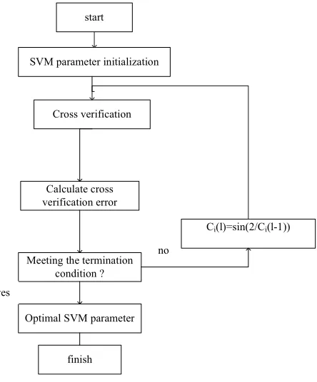
of quantum particle swarm optimization. The process of chaos searching is as follows and its flow chart is Fig. 1.

Step1.

i

=

0

and

i

is label of chaos searching of particle swarm.

Step2. Do chaos searching to the i-th dimension of

P

_g.

(1)Iteration time

l

=

0

and chaos variable

C l

i

( )

belonging to

[ 1,1]

−

is generated randomly which does not

include chaos fixed point.

(2)If

C l

_i

( )

>

0

, (9) sets up. Otherwise (10) sets up.

( )

2 ( )

(

( )

)

( )

gi gi i gi

i

gi gi i

P

P C l

P

Xup i

P

Xup i

P C l

other

+ ⋅

⋅ <



=



+

− ⋅



. (9)

(

( ))

( )

i gi gi i

P

=

P

+

P

−

Xdown i

⋅

C l

. (10)

If

f P

( )

_i

<

Gbsetfitness

,

Gbsetfitness

=

f P

( )

_i ,

P

_gi

=

P

_i.

(3)

l

= +

l

1

,

C l

_i

( )

=

sin(2 /

C l

_i

(

−

1))

.

(4)Repeat (2) and (3) until given maximum chaos iteration time

N

_c comes. Step3.

i

= +

i

1

Step4. Return to step 2 to recalculate until all dimensions of particle experience chaos searching.

The proposed new particle swarm algorithm based on chaos searching and extreme disturbance is as follows and its flow chart is Fig. 2.

Step1.Iteration time

k

=

0

and maximum chaos iteration time

N

_c is established. Position of each particle in the swarm is initialized.

Step2. Calculate fitness of each particle according to objective function

f

_i.

Step3. Update individual optimal fitness

Pbestfitness

and individual optimal position

P

_i.

Step4. According to

PIterCount

determine whether the particle stops. If it stops, then do individual extreme disturbance. Otherwise turn to step 5.

Step5. Update global optimal fitness

Gbestfitness

and global optimal position

P

_g.

Step6. According to

GItercount

determine whether the swarm stops. If it stops, then do global extreme disturbance and turn to step 7.

Step7. Calculate swarm fitness variance

σ

2. If

σ

2

<

T

, do chaos searching and turn to step 8. Step8. Calculate new position of each particle according to (1), (2) and (3).

(5)

______________________________________________________________________________

III. ANEWNETWORK TRAFFIC PREDICTION SCHEMEBASEDONCHAOSPARTICLESWARMSVM

Parameters selection of SVM is a kind of combinatorial optimization problem and is the search for an optimal solution in search space. Parameter optimization process of SVM based on intelligent algorithm is as follows and its flow chart is Fig. 3.

Step1. Within given parameter range, produce

N

number of particles randomly, which is

N

groups of SVM parameters

( , , )

ε

C

γ

. Use real coding so that we need randomly initialize within the area of solution.

Step2. Calculate fitness of each particle.

(1) For each particle training set

( ,

x y

_i _i

)

, with

n

number of samples is divided into

k

number of subset

1

,

2

,

k

G G

L

G

,

i

=

1, 2,

L

,

n

.

(2)

G

_i groups of samples are used to check and other subsets are used to train SVM. Error is calculated by (11).

j

y

is the actual value and



y

_j is output value.



2

[

]

i j i

G j j

y G

E

y

∈

=

∑

−

. (11)

(3) repeat (2) from

G

₁ until

k

groups of data are checked. (4) Calculate fitness of particle using (12).

1

i

k G i

fitness

E

n

=

∑

. (12)

Step3. According to the process of improved particle swarm optimization based on chaos, go on the iteration until meeting the termination condition.

ε

γ

(6)

set up model according to different characteristics to simplify complex issues. Considering sequence after the

α

Trous wavelet transform of the sequence can establish direct contact at the time point of each time scale, which has the time shift invariance and better generalization ability of support vector machine (SVM). This paper proposes a network traffic prediction model based on wavelet transformation and optimized SVM.

start

SVM parameter initialization

Cross verification

Calculate cross verification error

Ci(l)=sin(2/Ci(l-1))

Meeting the termination condition ?

Optimal SVM parameter

finish

no

[image:6.595.200.422.129.397.2]

yes

Figure 2. Parameter optimization process of proposed scheme

Figure 3. Architecture of network traffic prediction

Architecture of network traffic prediction is shown in Fig .3. The detailed prediction process is as follows.

Step1. Wavelet decomposition and reconstruction. The choice of wavelet base and wavelet decomposition series have an impact on forecasting accuracy. Wavelet decomposition series L is neither too small nor too big. Too small L can't effectively isolate different frequency characteristics of the network traffic. Too big L can result in model prediction error accumulated to the final forecasting result, which lower prediction accuracy and also can increase the computational complexity. So we should choose suitable wavelet base and decomposition series to decompose network traffic data into wavelet coefficients

d d

₁

,

₂

,

L

,

d

_L_{and scale coefficient}

L

(7)

______________________________________________________________________________

Step2. Data processing. Due to the bigger change range of the data, in order to improve the prediction accuracy, each signal component is normalized.

$

min( )

max( ) min( )

i

i i

x

−

=

−

. (13)

After normalization

$

x

∈

[0,1]

.

Step3. Model initialization. Determine the training set and test set, according to minimum cross validation error criterion choose a suitable embedding dimension

m

for each coefficient component. Input vector and output vector of SVM prediction model are obtained according to embedding dimension

m

.

Step4. Determination of SVM model. The processed signal through wavelet transform is approximately smooth in the high frequency part. This portion of the signal can be predicted using the traditional linear model. But the complexity of network traffic requires constantly adjusting the model parameters in order to adapt to the changing of the flow condition. Parameter optimization of SVM is based on improved chaos particle swarm.

Step5. SVM training and prediction. We adopt minimum sequence algorithm. Step6. Each prediction result is normalized inversely according to (14).

$

[max( ) min( )] min( )

_i _i _i

x

= ⋅

x

−

x

+

x

. (14)

Then do wavelet reconstruction to get the final prediction of network traffic.

IV. EXPERIMENT RESULTS AND ANALYSIS

A. Rough time granularity network traffic prediction

Experimental platform is matlab7.0. In order to evaluate prediction performance, this paper we choose root mean square error as performance index.



2 1

1 (

)

n

i i

i

RMSE

y

n

=

∑

−

. (15)

i

y

is the real value and



y

_i is prediction value. The smaller the

RMSE

, the better the prediction performance. Rough time granularity network traffic data comes from http://newsfeed.ntcu.net/~news/2006, which collected a total of 43 days network traffic per hour of primary node router. There are 1032 rough time granularity data. 240 data of the first 10 days is taken as training set and 792 data of the last 33days is taken as testing set. Basic parameter of chaos particle swarm optimization SVM is shown in TABLE I and TABLE II.

TABLE I- parameter of chaos particle swarm optimization SVM

[image:7.595.64.545.602.650.2]

Coefficient component Population size Maxiter

N

_c

T

_p

T

_g Scale coefficient 20 12 10 4 5 Wavelet coefficient 20 12 10 4 5 TABLE II parameter of chaos particle swarm optimization SVM

RBF core parameter

γ

parameter Sigmoid core

k

Sigmoid and Polynomial core parameter

v

Polynomial core

parameter

d

c

ε

[0.01,3] [0.001,1] [0,1] 2 [0.1,1000] [0.001,0.1]

[0.01,3] [0.001,1] [0,1] 2 [0.1,1000] [0.006,0.1]

TABLE III model prediction performance under different wavelet decomposition series

Decomposition serial 1 2 3 4 5

(8)

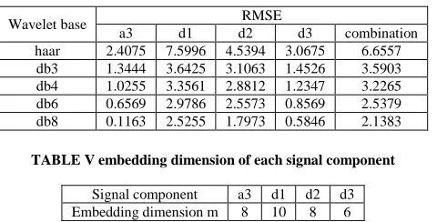
TABLEIVmodel prediction performance under different wavelet base

Wavelet base RMSE

[image:8.595.189.429.87.209.2]

a3 d1 d2 d3 combination haar 2.4075 7.5996 4.5394 3.0675 6.6557 db3 1.3444 3.6425 3.1063 1.4526 3.5903 db4 1.0255 3.3561 2.8812 1.2347 3.2265 db6 0.6569 2.9786 2.5573 0.8569 2.5379 db8 0.1163 2.5255 1.7973 0.5846 2.1383 TABLE V embedding dimension of each signal component

Signal component a3 d1 d2 d3 Embedding dimension m 8 10 8 6

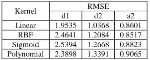
TABLE III is model prediction performance under different wavelet decomposition serials. When decomposition becomes from 1 level to 3 level, RMSE decreases quickly and later RMSE decreases slowly. Considering the computation complexity and prediction accuracy, the traffic data is decomposed into 3 levels. TABLE IV gives the model prediction performance under different wavelet base. We can see that prediction performance of db8 wavelet base is better than other wavelet base. So in this paper, we adopt db8 wavelet base to decompose network traffic data into 3 levels. Then we obtain corresponding wavelet coefficient d1, d2, d3 and scale coefficient a3. TABLE V is embedding dimension of each signal component. TABLE VI is prediction performance contrast under different core function after db8 wavelet decomposition. We can see that Linear core SVM is better than other core SVM and in scale coefficient layer, RBF core SVM has better performance. We compare the performance of proposed algorithm with other prediction models including SVM model, model based on wavelet transformation and BP naming WaBPNN, WFIRNN and WaSVM using standard particle swarm optimization to optimize its parameters. Input node of BP of each signal component is the same with embedding dimension m. Number of hidden layer node is 12. Order of FIR is

12 2

×

and number of output node is 1. We do 20 times experiment to acquire mean value of RMSE. TABLE VII is SVM model optimization parameter of each layer. TABLE VIII is prediction performance contrast of different model.

TABLE VI model prediction performance under different core function

Kernel RMSE

d1 d2 d3 d4

[image:8.595.162.451.510.577.2]

Linear 2.2594 1.2693 0.5605 0.2185 RBF 2.5255 1.7973 0.5846 0.1163 Sigmoid 2.4742 1.8569 0.5911 0.2531 Polynomial 2.6367 1.7281 0.6125 0.2593 TABLE VII SVM model optimization parameter of each layer

Coefficient component Chaos searching threshold T

γ

SVM parameter

_c

ε

a3 2e-7 0.321 544.949 0.0013

d1 1e-7

×

837.359 0.0176

d2 3e-7

×

279.916 0.0169

d3 5e-7

×

292.234 0.0131

TABLEVIIIprediction performance comparison of different model

Model RMSE

a3 d1 d2 d3 combination

SVM

×

14.1358

(9)

______________________________________________________________________________

It can be seen that prediction of SVM model is the largest. Wavelet neural network is easy to trap into local optimization. In a word, prediction accuracy of ChOSVM is better than other models.

B. Fine time granularity network traffic prediction

TABLE IXembedding dimension of each signal component

[image:9.595.155.452.117.432.2] [image:9.595.231.382.194.255.2] [image:9.595.163.448.275.435.2]

Signal component a2 d1 d2 Embedding dimension m 7 10 8

TABLE Xprediction performance comparison of different model

Kernel RMSE

d1 d2 a2

Linear 1.9535 1.0368 0.8601 RBF 2.4641 1.2084 0.8517 Sigmoid 2.5394 1.2668 0.8823 Polynomial 2.3898 1.3391 0.9065

TABLE XI SVM model optimization parameter of each layer

Coefficient component Chaos searching threshold T

γ

SVM parameter

_c

ε

a2 5e-8 0.689 570.035 0.0021

d1 3e-7

×

540.869 0.0172

d2 5e-8

×

634.083 0.0151

TABLE XIIprediction performance comparison of different model

Model RMSE

A2 d1 d2 combination

SVM

×

16.4367

WaBPNN 2.1861 8,8132 3.7541 7.2794 WFIRNN 1.1861 5.9354 2.1962 4.1478 WaSVM 0.9065 2.4612 1.2967 1.9763 ChOSVM 0.8586 1.9535 1.0368 1.5958

Fine time granularity network traffic data comes from http://ita.ee.lbl.gov/html/contrib/BC.html.We choose BC-Oct89Ext data set. Traffic data is transformed into 500 traffic data. The first 200 data is taken as training set and the last 300 data is taken as testing set. We adopt db8 wavelet base to decompose traffic data to 2 level. Embedding dimension of each signal component is shown in TABLE IX. TABLE X is prediction performance contrast under different core function after db8 wavelet decomposition. We can see that Linear core SVM is better than other core SVM and in scale coefficient layer, RBF core SVM has better performance. SVM model optimization parameter is shown in TABLE XI and prediction performance comparison of different model is shown in TABLE XII. We compare the performance of proposed algorithm with other prediction model including SVM model. It can be concluded that prediction accuracy of ChOSVM is better than other models.

CONCLUSION

Network traffic shows obvious multi-scale characteristic, which is composed of different signals and different components have different inherent law. Based on the complex characteristics of network traffic, this paper puts forward a network prediction model based on wavelet decomposition and scale coefficient. The results show that the optimized SVM has better generalization ability, ChOSVM can achieve ideal prediction accuracy only using a small number of training samples and its performance is obviously better than the single SVM model and some existing combination forecasting model. It has good robustness and strong generalization ability and high prediction accuracy.

REFERENCES

[1] Xiaoling Tan, Weijian Fang, Yong Qu, International Journal of Advancements in Computing Technology, Vol. 5, No. 5, pp. 183-190, 2013.

(10)

[4] G. He, Y. Gao, J. C. Hou, and K. Park, “A case for ex-ploiting self-similarity of Internet traffic in TCP congestion control,” In Proc. IEEE ICNP, Nov. 2002.

[5] H. Tong, C. Li, and J. He, “A boosting-based frameworkfor self-similar and non-linear Internet traffic prediction,”In Proc. of International Symposium on Neural Networks (ISNN ), August 2004.

[6] Y. Xinyu, Z. Ming, Z. Rui, and S. Yi, “A novel LMS method for real-time network traffic prediction,” In Proc. of Computational Science and Its Applications (ICCSA), May 2004.

[7] F. Rouai and M. Ahmed, INNS-IEEE International Joint Conference on Neural Network (IJCNN), vol. 2, 2001. [8] N. Sadek and A. Khotanzad, Proceedings of IEEE International Joint Conference on Neural Networks, vol. 3, July 2004. pp. 2407–2412.

[9] A.-M. Yang, X.-M. Sun, C.-Y. Li, and P. Liu, “A neuro-fuzzy method of forecasting the network traffic of ac-cessing web server,” 2nd International Conference on Fuzzy Systems and Knowledge Discovery, Lecture Notes in Computer Science, vol. 3613, August 2005.

[10]M. Çınar, M. Engin, E. Z. Engin and Y. Z. Ateşçi, Expert Sys-tems with Applications, Vol. 36, No. 3, 2009, pp. 6357- 6361.

[11]D.-C. Park, “Structure Optimization of Bi-Linear Recur-rent Neural Networks and its Application to Ethernet Network Traffic Prediction,” Information Sciences, 2009, in press.

[12]B. R. Chang and H. F. Tsai, Applied Soft Computing, Vol. 9, No. 3, 2009, pp. 1177-1183. [13]R. Yunhua, Computer Communica-tions, Vol. 27, No. 9, 2004, pp. 898-904.

[14]B. C. Lu, M. L. Huang, “Traffic Flow Prediction Based on Wavelet Analysis, Genetic Algorithm and Artificial Neural Network,” in Proc. of the International Conference on Information Engineering and Computer Science (ICIECS), Wuhan, 2009, pp. 1–4.

[15]X. Y. Yang, S. S. Yang, J. Li, Chinese journal of computers, vol. 34, no. 2, pp. 395–405, 2011. [16]M. Jiang, et al, Acta Electronic Sinica, vol. 37, no. 11, pp. 2353–2358, 2009.

[17]X. T. Chen, J. X. Liu, Journal on communications, vol. 32, no. 4, pp. 153–157, 2011.

[18]H. L. Sun, Y. H. Jin, Y. D. Cui, S. D. Cheng, Journal of Beijing University of Posts and Telecommunications, vol. 33, no. 1, pp. 7–11, 2010.

[19]L. Zhu, L. Qin, K.Y. Xue, X.Y. Zhang, “A Novel BP Neural Network Model for Traffic Prediction of Next Generation Network,” in Proc. of the Fifth International Conference on Natural Computation (ICNC 09), Tianjian,

2009, pp. 32–38.

[20]Q. F. Yao, C. F. Li, H. L. Ma. S. Zhang, Journal of Zhejiang University (science ed.), vol. 34, no. 4, pp. 396– 400, 2007.

[21]P. Wang, S. Y. Zhang, X. J. Chen, “SFARIMA: A New Network Traffic Prediction Algorithm,” in Proc. of the 1st International Conference on Information Science and Engineering (ICISE), Nanjing, 2009, pp. 1859–1863. [22]Y. M. Mao, S. Y. Shi, “Research on Method of the Subsection Learning of Double-Layers BP Neural Network in Prediction of Traffic Volume,” in Proc. of the International Conference on Measuring Technology and Mechatronics Automation (ICMTMA 09), Zhangjiajie, 2009, pp. 294–297.

[23]M. Dusi, A. Este, F. Gringoli, L. Salgarelli, “Using GMM and SVM-Based Techniques for the Classification of SSH-Encrypted Traffic,” IEEE International Conference on Communications, Dresden, 2009, pp. 1– 6.

[24]C.J. Gu, S.Y. Zhang, Chinese Journal of Scientific Instrument, , vol. 32, no. 7, pp.1507-1513, 2011.

[25]E. Alice, G. Francesco, S. Luca, The International Journal of Computer and Telecommunications Networking, vol. 53, no.14, pp. 2476-2490, 2009.

[26]Shu Fan, Fengchun Tian, Qinghua He, Pengfei Jia, Jingwei Feng, Yue Shen, Journal of Convergence Information Technology, 2012, Vol. 8, No. 5, pp. 1209-1219.

[27]Youxin LUO, Xiaoyi CHE, Lingfang LI, Journal of Convergence Information Technology, 2012, Vol. 7, No. 22, pp. 484-491.