Modeling and control of 6 DOF industrial robot using fuzzy logic controller

MODELING AND CONTROL OF 6 DOF INDUSTRIAL ROBOT USING FUZZY LOGIC CONTROLLER

DZULHIZZAM BIN DULAIDI

A thesis is to submitted in

fulfillment of the requirement for the award of Degree of Master Electrical Engineering

Faculty of Electrical and Electronics Engineering Universiti Tun Hussein Onn Malaysia

ABSTRACT

ABSTRAK

CONTENTS

TITLE i

DECLARATION ii

DEDICATION iii

ACKNOWLEDGEMENT iv

ABSTRACT v

CONTENTS vii

LIST OF TABLE ix

CHAPTER 1 INTRODUCTION 1

1.1 Motivation 1

1.2 Problem Statement 2

1.3 Aim and Objective 3

1.4 Scope of Project 3

1.5 Project Planning 4

CHAPTER 2 LITERATURE REVIEW 5

2.1 Background 5

2.1.1 Control Techniques 8

2.2 Robot Controller 10

2.3 Robot Kinematics 12

2.3.1 Forward Kinematics 12

2.4.1 PID Structure 16

2.4.2 PID Characteristics Parameters 18

2.5 Fuzzy Logic Controller 18

2.5.1 Fuzzy Logic Theory 19

2.5.2 Parameters Identification in Fuzzy Modeling 20

2.5.3 Fuzzification 21

2.5.2 Defuzzification 23

CHAPTER 3 METHODOLOGY 24

3.1 Introduction 25

3.2 Modeling in SolidWorks 25

3.2.1 Robot Kinematics 28

3.3 Modeling and Designing of FLC 29

3.3.1 Rule Base Derivation 32

3.4 DC Motor Modeling 33

CHAPTER 4 RESULTS AND DISCUSSIONS 37

4.1 Introduction 37

4.2 KUKA R5 Case Study 37

CHAPTER 5: CONCLUSION AND RECOMMENDATION

5.1 Conclusion 48

5.2 Recommendation 49

REFERENCE 50

LIST OF TABLES

Table 2.1: D-H Parameter for Robot Manipulator in Figure 2.5 14

Table 2.2: PID characteristics parameters 18

Table 3.1: DH parameters of KUKA R5 robot arm 27

Table 3.2: Table of Fuzzy Rule 30

Table 3.3: Rule base for fuzzy controller 32

Table 3.4: DC motor parameter and value 36

Table 4.1: End effector home position {0°,0°,0°,0°,0°,0°} 40 Table 4.2: Endeffector position with input angle

θ = {45° ,-90°,45°, -90° ,45°,45} 40

LIST OF FIGURES

Figure 2.1: Robot manipulator with joints and links 6

Figure 2.2: Closed Loop (CL) block diagram 7

Figure 2.3: Robotic movement system with fuzzy logic

controller block 11

Figure 2.4: D-H Frame Assignment 13

Figure 2.5: Robot Manipulator with 5-links 14

Figure 2.6: Typical PID control structure 17

Figure 2.7: PID parallel form structure 17

Figure 2.8: Fuzzy Controller Block Diagram 19

Figure 2.9: Triangular membership functions over value

range [x_min,x_max] of an input variable x. 21

Figure 2.10: Fuzzy sets defining temperature 22

Figure 2.11: Defuzzification method 23

Figure 3.1: KUKA R5 overview 26

Figure 3.2: Frame assignment for the KUKA R5 robot arm 26 Figure 3.3: Solidworks modeling of KUKA R5 robot arm 27

Figure 3.4: Fuzzy inference block 30

Figure 3.5 (a): Fuzzy input variable, error (e) 31

Figure 3.5 (b): Fuzzy input variable, change of error (∆e) 31

Figure 3.6: Fuzzy output variable 32

Figure 3.7: DC motor systems 34

Figure 4.1: KUKA R5 Joint and Link in SIMULINK/MATLAB 38 Figure 4.2: Fuzzy and PID Controller in

MATLAB/SIMULNIK to Control θ1 38

Figure 4.3: Fuzzy and PID Controller in

Figure 4.4: Fuzzy and PID Controller in

MATLAB/SIMULNIK to Control _θ3 39

Figure 4.5: Fuzzy and PID Controller in

MATLAB/SIMULNIK to Control _θ4 39

Figure 4.6: Fuzzy and PID Controller in

MATLAB/SIMULNIK to Control θ5 39

Figure 4.7: Fuzzy and PID Controller in

MATLAB/SIMULNIK to Control θ6 39

Figure 4.8: Home position for the KUKA R5 40

Figure 4.9: Endeffector position with input angle

θ = {45° ,-90°,45°, -90° ,45°,45} 41 Figure 4.10: PID and Fuzzy Controller Step Response for θ1 42 Figure 4.11: PID and Fuzzy Controller Step Response for _θ2 42 Figure 4.12: PID and Fuzzy Controller Step Response for θ3 42 Figure 4.13: PID and Fuzzy Controller Step Response for θ4 42 Figure 4.14: PID and Fuzzy Controller Step Response for _θ5 43 Figure 4.15: PID and Fuzzy Controller Step Response for θ6 43 Figure 4.16: Output with disturbance rejection θ1 45

Figure 4.17: Output with disturbance rejection θ2 45

LIST OF SYMBOLS AND ABBREVIATIONS

r, r(t) - Reference input

e, e(t) - Error between the input signal and the output u, u(t) - Input applied by the controller to plant y, y(t) - Output of the closed loop control system Gp (s) - Plant transfer function

Gc (s) - Controller transfer function

Gd (s) - Disturbance input to output transfer function H(s) - Feedback measurement

Dt (s) - Disturbance input

va (t) - Input source voltage, [Volt] vb (t) - The Back EMF

ia (t) - Armature current, [Ampere] Ra - Armature resistance, [Ohm] La - Electric inductance, [H] τ_{m -} Motor torque, [Nm] Km - Proportional constant

Kb - Back EMF constant, [V/ms-1] Kt - Motor torque constant, [Nm/A]

Jm - Moment of inertia of the rotor, [Kgm-1] θm - Rotor position, [rad]

φ - Magnetic flux, [Weber]

Bm - Coefficient of motor friction ωm - Angular speed, [rad/sec]

θi (t) - Joint angle for joint i of robot manipulator gr - Gear ratio

qi - Joint variable

Ai - Transformation matrix for joint i 0

n

H - _{Total transformation matrix} 1

i i

T − - _{Homogeneous transformation matrix of}

i relative to i-1 KP - Proportional gain

KD - Derivative gain KI - Integral gain

TI - Integral time constant TD - derivative time constant tr - Rising time, [sec] ts - Settling time, [sec] µ(u) - Membership function

Φ - Null fuzzy set (Phi)

∆e - Change of the error ke - Scaling factor for error

kde - Scaling factor for change of error ku - Scaling factor for output

n - Degree of freedom of robot manipulator (n-DOF robot manipulator)

i - Number of links

R - Number of the fuzzy rules

BOA - Bisector of Area

COA - Centroid of Area

CL - Closed Loop

DOF - Degree of Freedom

DH - Denavit Hartenberg

DC - Direct Current

EMF - Electromagnetic Force

FK - Forward Kinematic

FLC - Fuzzy Logic Controller

IK - Inverse Kinematic

LOM - Largest of Maximum

MM - Maximum Method

CHAPTER 1

INTRODUCTION

1.1 Motivation

Industrial robot manipulator field is one of the interested fields in industrial, educational and medical applications. Research in control the motion and movement of industrial robot was the most concentrate field during recent year.

Due to advance computer and visualization technology, robotic manipulator study are divided in two categories, mathematical modeling and computer modeling of the manipulator and the actuators, which includes an analysis for the forward kinematic, the inverse kinematic and modeling the direct current motor.

This study is focus on modeling an industrial robot manipulator and designing controller for the motion of the industrial robot manipulator meet the requirement of the desired trajectory or desired angle.

1.2 Problem Statement

Motion control is fundamental to many robotics applications, and is known to be a difficult problem. Execution in real world environments is confounded by noisy sensors, approximate world models and action execution uncertainty. A practical and mathematical model of industrial robot required many equations and consumed much time when it comes to design and experiment a real model. It has been proved that the benefit of design an industrial model in computer simulation had reduced the cost and time in designing and simulates an industrial robot [8].

The complexity of the robotic tasks is getting more and more advanced, so an intelligent, robust, computationally simple and easy to implement controller must be designed and analyzed to optimize and maximize the performance of industrial robot [6].

The problem statements of this study are:

i. Robot system and its mathematical modeling is very complex system, a computer software simulation is the easiest method to model a real robot without writing a code/programming and derive mathematical equation. ii. Performing an experiment a behavior and mechanism of a real robot may

damage the robot and required lot of money, a robot modeling and computer simulation required to reduce the cost and time to study a robot system.

iii. PID controller is not sufficient to obtain the desired tracking control performance because of the nonlinearity of the robot manipulator, so nonlinear controller such as Fuzzy Logic is required to minimize and counter the nonlinearity issue.

1.3 Aim And Objectives

To model and design the controller for a 6 DOF of industrial robot is the aim of this research. The industrial robot should be able to perform and simulate a pick and place task in MATLAB/SIMULINK environment. To achieve these aims, the objectives of this research are formulated as follows:

i. To design a 6 DOF of industrial robot model by using CAD software.

ii. To apply and tune a PID controller to the 6 DOF of industrial robot as a benchmarking controller.

iii. To design a controller using Fuzzy Logic approach for the 6 DOF of industrial robot.

iv. To compare the performance of the Fuzzy Logic Controller with the PID controller.

1.4 Scope Of Project

This project embarks based on the following scopes:

i. Design and modelling industrial robot by using SolidWork software.

ii. The simulation study and analysis the performances and the effectiveness of PID and Fuzzy controller using MATLAB/SIMULINK environment.

1.5 Project Planning

No.

YEAR 2013 2014

MONTH APRIL MEI JUN JUL OGOS SEPT OCT NOV DEC JAN

Description

PROJECT 1

1 Literature review

2 Setting objective _{and scope}

3 Methodology

4 Apply PID method to Robot

Arm

5 Analyze overall system & data

collection

6 Draft project report & presentation

slide

7

Presentation & Proposal

submission

PROJECT 2

8 Design Fuzzy _{Logic Controller}

9 Simulation and _{analyzing the result}

10 Draft project report & slide

presentation

11

Seminar,

evaluation & thesis

submission

Legend

Complete task

CHAPTER 2

LITERATURE REVIEW

2.1 Background

Robot is a word from the Czech word robota, which means ‘slave laborer’. Czech

playwright Karel Capek (1890-1938) made the first use of the word ‘robot’ as a perfect, tireless worker with arms and legs. Referring to Robot Institute of America (RIA) a robot is "A reprogrammable, multifunctional manipulator designed to move material, parts, tools, or specialized devices through various programmed motions for the performance of a variety of tasks". According to Webster a robot is "An automatic device that performs functions normally ascribed to humans or a machine in the form of a human."

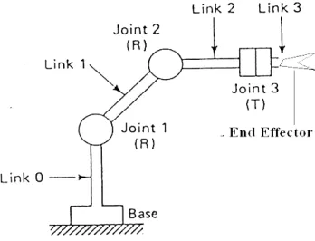
Number Degree of Freedom (DOF) which a manipulator possesses is the number of independent position variables that would have to be specified in order to locate all parts of the mechanism. In different words, it refers to the number of different ways in which a robot arm can move. In the case of typical industrial robots, because a manipulator is usually an open kinematic chain, and because each joint position is usually defined with a single variable, the number of joints equals the number of degrees of freedom.

There are two widespread types of joints on this manipulator. The first type is called revolute or rotary joint (e.g. human joints), it allows only relative rotation between two links. This type of joint is and it is the most common joint type in robots. The second type of joints is called prismatic or slidingjoint. This type of joints allows only linear relative motion between two links along its axis. Both types are denoted as R and P joints.

Figure 2.1: Robot manipulator with joints and links

Classification of robot manipulators is categories by types of coordinate systems. Normally, robot manipulators are classified according to their arm geometry or kinematics structure. The majority of these manipulators fall into one of these five configurations: Cartesian (PPP), Cylindrical (RPP), Spherical (RRP), SCARA (RRP), Articulate/Revolute (RRR). Robot manipulator in Figure 2.1 is called revolute revolute revolute (RRR) manipulator and also referred as Articulate/Revolute manipulator.

Control system in robot manipulators is very important to control and adjust the robot manipulator. Generally, two types of control systems are used: the open loop (OL) control system and closed loop (CL) control system. In OL control system, the controller sends a signal to the motor but does not measure the error action. On other hand, in CL control system, the controller sends the signal to the motor, and the output signal will be returned as feedback to describe the current state of the motor. CL controller has some advantages over the OL controller such as: disturbance rejection like friction in motors, improve reference-tracking performance and stabilization of an unstable process.

moving, the robot manipulator during the working environment, the sensor or feedback system is gathering the information about the robot manipulator state and the surrounding circumstances, and then exploiting the information to modify and enhance the system behavior. Control system provides some function for the plant (robot arm) such as: a) providing the capability to move the robot manipulator in the surrounding environments. b) Collecting information about the robot manipulator in the working place. c) Using this information to give a methodology to control the robot manipulator. d) Storing the data then providing it to the robot manipulator then updating it at an instant.

One of the most vital and powerful issues in robotic fields is the control motion of the manipulator, because the robot operation must be accurate, without any effect in surrounding circumstances. Controlling manipulators is a major research area to limit the time history of joint inputs that required moving the end-effector to execute the required mission.

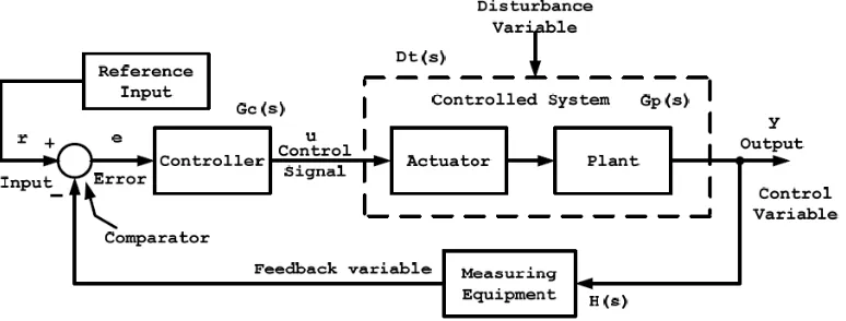
Figure 2.2: Closed Loop (CL) block diagram

The basic configurations of the closed-loop control system depicted in Figure 2.2 include some main building components. The closed loop control system consists of the reference input or the set point of the closed loop, r(t) , summer, controller, the

controlled plant, the output or the measured value y(t) , and the feedback loop. The plant, Gp(s) , is the physical system (e.g. a robot manipulator); it includes the actuators, gears,

and mechanical design. The controller Gc(s), is a device which is used to correct the

error signal e(t) = r(t) - y(t) and supply appropriate input to modify the physical system

The controller attempts to reduce the error between the set point and the feedback signal to zero. However, if the input signal and feedback signal are not equal, the controller will correct the position signal until the difference between both signals is zero. Some disturbance variables Dt(s), may influence the output signal. These

disturbances are unpredictable inputs. The sensor H(s), is the device that measures the

output signal. Many systems may be unstable at all times due to nonlinearity, so a good control system must produce control output to track the desired response. This confirms that the important issue in designing a control system is to ensure that the dynamic response of the closed loop systems is stable.

2.1.1 Control Techniques

Many control techniques have been proposed to control robot manipulator ranging in complexity from linear to the advanced control system, which compute the robot dynamic and save it from damage in real environments. Three different control schemes namely Proportional-Integral-Derivative (PID) controller, and Fuzzy Logic Controller (FLC) will be implemented in this study. The performance of these controllers will be based on the high precision in reducing the overshoot, minimizing steady state error, damping unwanted vibration of robot manipulator, and handling the unpredictable disturbances.

Hence, a lot of time is required to tune the PID parameters. On the other hand, other techniques are used to overcome the previous problem, such as fuzzy controller that emulates human operation.

FLC is an emerging technique in control systems. It is considered as intelligent controller. Many studies show that the fuzzy controller (FC) performs superior to conventional controller algorithms. Zadeh [8] did the main idea of FLC and fuzzy set theory. Mamdani and his colleagues [9] have done a pioneering research work on FLC in the for engine steam boiler. The benefit of FLC is obvious when the controlled process is too complicated to be analyzed using PID controller or when the information about the controlled system does not exist.

FLC is classified into two categories: the first, involves the fuzzy logic system based on a rule based on expert system, to determine the control action. The second used FL to provide online adjustment for the parameters of the conventional controller such as the PID control [10]. This method attempts to combine the merits of FL with those control techniques to expand the capability of linear control technique to handle the nonlinearity in the physical system. Fuzzy supervisory is used to reduce the amount of tuning the PID controller with a fuzzy system [11]. It is considered as an attractive method to solve the nonlinear control problems, one of the advantages of fuzzy supervisory that the control parameters changed rapidly with respect to the variation of the system response.

2.2 Robot controller

Several of studies and research have been done in industrial robot disciplines. The studies on the industrial robot focused on the kinematics analysis of industrial and educational robots. Some other papers discussed control technique in industrial robot such as PID and Fuzzy Logic.

In robot simulation, system analysis needs to be done, such as the kinematics analysis where its purpose is to carry through the study of the movements of each part of the robot mechanism and its relations between itself. Kinematics analysis is essential for robotic design and control. The kinematics analysis is divided into forward and inverse analysis. Industrial robot kinematics mathematical model is using Denavit-Hartenberg (D-H) method [9]. This method was introduced by Jacques Denavit and Richard S. Hartenberg [2]. In D-H algorithm, coordinate frames are attached to the joints between two links such that one transformation is associated with the joint, and the second is associated with the link. The coordinate transformations along a serial robot consisting of n links form the kinematics equations of the robot.

In Elgazzar research paper, the efficient solutions for the kinematic positions, velocities, and accelerations for the six-degree-of-freedom PUMA 560 robot are presented [10]. The kinematic problem is defined as the transformation from the Cartesian space to the joint space and vice versa. The solution method is based on a method that fully exploits the special geometry of the robot in the derivation of the solution. Special attention is given to the arm configuration in both directions of the transformation. In this paper Elgazzar concluded that for any six-degree-of-freedom robot with a spherical wrist, the solution of the first three joints depends on the given robot, whereas the solution of the last three joints (forming the spherical wrist) is independent of the robot.

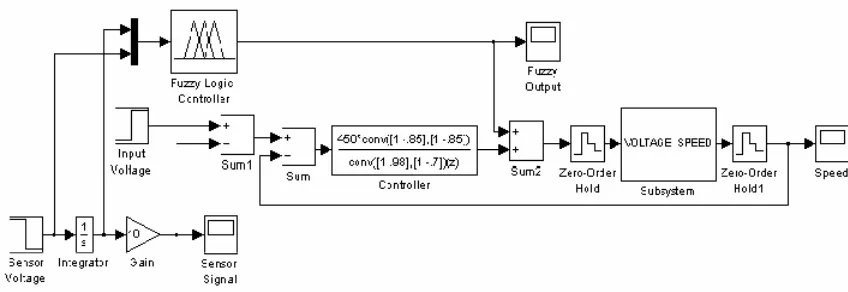
speed and increases the stability of the system. Figure 2.3 shows the fuzzy controller block diagram in MATLAB/SIMULINK.

Figure 2.3: Robotic movement system with fuzzy logic controller block

Khoury presented the design of a fuzzy logic controller of 5 DOF robot arm [8]. Through his paper, he introduced two structures of FLC: first three inputs with coupled rule base and the second structure was two inputs with coupled rules. Khoury confirmed the success of the proposed fuzzy controller. Compare to the conventional controller such as PID fuzzy controller tracking capabilities is more efficient and precise [15].

Comparison between FLC and PID Controller for 5 DOF of Robot Arm by Alassar and Abuhadrous [16] found that Fuzzy provides good results than PID controller. The research results based on the eliminating the overshoot, achieving zero steady state error, damping the unwanted vibration of the industrial robot, and handling the unpredictable disturbances using controller techniques. A lot of time requires tuning PID due to its insufficient to obtain the desired tracking control performance because of the nonlinearity of the industrial robot due to unpredictable environment.

2.3 Robot Kinematics

Kinematics is the analytical study of the geometry of motion of a robot arm: with respect to a fixed reference co-ordinate system without regard to the forces or moments that cause the motion.

The kinematics analysis is divided into forward and inverse analysis. The forward kinematics consists of finding the position of the end-effector in the space knowing the movements of its joints as F ( ߠ_ଵ, ߠ_ଶ,… ߠ_௡, ) = [x, y, z, R], and the inverse

kinematics consists of the determination of the joint variables corresponding to a given end-effector position and orientation as F[x, y, z, R]=( ߠ_ଵ, ߠ_ଶ,… ߠ_௡,).

2.3.1 Forward Kinematics

Forward kinematics refers to the use of the kinematic equations of a robot to compute the position of the end-effector from specified values for the joint parameters. The kinematics equations of the robot are used in robotics, computer games, and animation.

In robot simulation, system analysis needs to be done, such as the kinematics analysis, its purpose is to carry through the study of the movements of each part of the robot mechanism and its relations between itself.

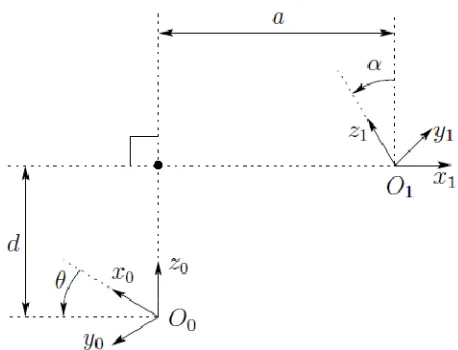
A commonly used convention for selecting frames of reference in robotic applications is the Denavit-Hartenberg or D-H convention as shown in Figure (2.4). In this convention each homogenous transformation H _i is represented as a product of

"four" basic transformations as below:

( , ) ( , ) ( , ) ( , )

i i i i i

Figure 2.4: D-H Frame Assignment

Where the notation Rot x( , )α_i stands for rotation about x_i axis by α_i ,

( , )_i

Trans x a is translation along x_i axis by a distance a_i, Rot z( , )

θ

about z_i axis by

θ

1 1

1 1 1 1

1 1

0 0 1 0 0 0 1 0 0 1 0 0 0

0 0 0 1 0 0 0 1 0 0 0 0

0 0 1 0 0 0 1 0 0 1 0 0 0

0 0 0 1 0 0 0 1 0 0 0 1 0 0 0 1

0

i

i

i

i i i i i i i

i i i i i i i

i

i

c s a

s c c s

H

d s c

c s c s s a c

s c c c s a s

H

s c

θ θ

θ θ α α

α α

θ θ α θ α θ

θ θ α θ α θ

α α −                    ₋            =                               − − =

0 0 0 1

i di

 

 

 

 

 

  _(2.2)

Where the four quantities

θ

various parameters in previous equation are given the following names:

i

a (Length) is the distance from z to _i z_i+1 , measured along z ;_i

i

α (Twist), is the angle between z to _i z_i+1 , measured about x_i ;

i

d (Offset), is the distance from x to _i x_i+1 , measured along z_i ; and

i

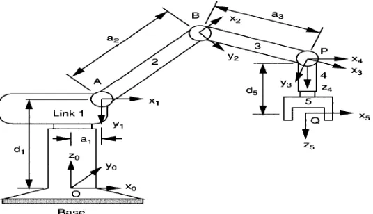
Robot manipulator in Figure 2.5 has a five link arm that starts out aligned in the x-axis. Each link has lengths a1, a2, a3, a4 respectively. First link move by θ1 , second

link move by θ2, third link move by θ3, fourth link move by θ4, and fourth link move by θ5as the diagram suggests.

The kinematic model is shown in Figure 2.5 is assigned with its frame assignments according to the Denavit & Hartenberg (D-H) notations. The kinematic parameters according to this model are given in Table 2.1.

Figure 2.5: Robot Manipulator with 5-links

Table 2.1: D-H Parameter for Robot Manipulator in Figure 2.5

Joint ࢏ Twist Angle, ࢻ_࢏ Link Length, ࢇ_࢏

(mm)

Joint Distance, ࢊ_࢏ (mm)

Joint Angle, ࣂ_࢏

1 ߙ_ଵ a1 d1 ߠ_ଵ

2 0 a2 0 ߠ_ଶ

3 0 a3 0 ߠ_ଷ

4 ߙ_ଶ 0 0 ቀߨ

2ቁ + ߠସ

5 0 0 d5 ߠ_ହ

1 1 1 1 1 1 1

1 1 1 1 1 1 1

1 0

1 1 1

0

0 0 0 1

c s c s s a c

s c c c s a s

H

s c d

θ

θ α

θ α

θ

θ

θ α

θ α

θ

α

α

2 2 2 2 2 2 2

2 2 2 2 2 2 2

2 1

2 2 2

0

0 0 0 1

c s c s s a c

s c c c s a s

H

s c d

θ

θ α

θ α

θ

θ

θ α

θ α

θ

α

α

3 3 3 3 3 3 3

3 3 3 3 3 3 3

3 2

3 3 3

0

0 0 0 1

c s c s s a c

s c c c s a s

H

s c d

θ

θ α

θ α

θ

θ

θ α

θ α

θ

α

α

4 4 4 4 4 4 4

4 4 4 4 4 4 4

4 3

4 4 4

0

0 0 0 1

c s c s s a c

s c c c s a s

H

s c d

θ

θ α

θ α

θ

θ

θ α

θ α

θ

α

α

5 5 5 5 5 5 5

5 5 5 5 5 5 5

5 4

5 5 5

0

0 0 0 1

c s c s s a c

s c c c s a s

H

s c d

θ

θ α

θ α

θ

θ

θ α

θ α

θ

α

α

ܪ଴ହ = ܪ଴ଵ× ܪଵଶ× ܪଶଷ× ܪଷସ× ܪସହ (2.3)

2.4 PID Controller

survey for process control systems conducted in 1989, more than 90 of the control loops were of the PID type [17].

PID controller is considered the most control technique that is widely used in control applications. A huge number of applications and control engineers had used the PID controller in daily life. PID control offers an easy method of controlling a process by varying its parameters. PID works well in industrial applications such as slow industrial manipulators were large components of joint inertia added by actuators. Since the invention of PID control in 1910, and Ziegler-Nichols’ tuning method in 1942 [7] and [18], PID controllers became dominant and popular issues in control theory due to simplicity of implementation, simplicity of design, and the ability to be used in a wide range of applications. Moreover, they are available at low cost. Finally, it provides robust and reliable performance for most systems if the parameters are tuned properly.

Setting the PID parameters is called tuning. Other methods use the Nyquist curve plotting of the plant such as Ziegler-Nichols tuning method [18]. All of these tuning formulas need to know a prior knowledge about the system. PID control technique is used to control and enhance the system characteristics such as reducing the overshoot, speed up rising time, and eliminating the steady state error. Each one of the PID parameters has specific criteria to enhance the characteristics of the controlled system.

2.4.1 PID Structure

The term PID stands for Proportional-Integral-Differential control. Each of these P, I and D are terms in a control algorithm, and each has a special purpose. Sometimes certain of the terms are left out because they are not needed in the control design. This is possible to have a PI, PD or just a P control. It is very rare to have an ID control.

As shown in Figure 2.6, the error signal, e(t) , is the difference between the set

point, r(t) , and the process output, y(t) . If the error between the output and the input values

proportional to change in the error signal for a given proportional gain K ._P Mathematically

the output of the proportional controller is given as follows:

( ) P ( )

u t =K e t

Figure 2.6: Typical PID control structure

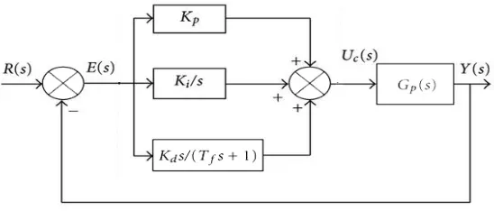
Figure 2.7 shows P, I, and D elements in parallel form, where all of them share a same input signal e(t) . The transfer function of the PID controller in parallel is:

2

( ) P D P I

PID P D

K K s K s K

G s K K s

s s

+ +

= + + =

(2.4)

Equation (2.4) may be rearranged to give the ideal form as follows:

1 1

( ) (1 )

PID P D

G s K T s

T s

= + +

(2.5)

where T_I =K_P /K_I and T_D =K_P /K_Dare the integral and derivative time constant

respectively.

2.4.2 PID characteristics parameters

Proportional action K _P improves the system rising time, and reduces the steady state

error. This means the larger proportional gain, the larger control signal become to correct the error. However, the higher value of K _P produces large overshot and the

system may be oscillating; therefore, integral action K I is used to eliminate the

steadystate error. Despite the integral control, reducing the steady state error, it may make the transient response worse [19]. Therefore, derivative gain K_Dwill have the

effect of increasing the damping in system, reducing the overshoot, and improving the transient response.

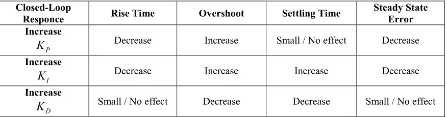
As discussed previously, each one of the three gains of the classical PID control has an effect of the response of the closed loop system. Table 2.2, summarizes the effects of each of PID control parameters. It will be known that any changing of one of the three gains will affect the characteristic of the system response.

Table 2.2: PID characteristics parameters

Closed-Loop

Responce Rise Time Overshoot Settling Time

Steady State Error Increase

P

K Decrease Increase Small / No effect Decrease

Increase

I

K Decrease Increase Increase Decrease

Increase

D

K Small / No effect Decrease Decrease Small / No effect

2.5 Fuzzy Logic Controller

very fast can be formulated mathematically and processed by computers, in order to apply a more human-like way of thinking in the programming of computers [4].

A fuzzy system is an alternative to traditional notions of set membership and logic that has its origins in ancient Greek philosophy. Control engineering is one of the major fields where the fuzzy theory has been successfully applied. Many researches and applications have been performed since Mamdani and his colleague [9] presented the first FLC work. Their work mimics the human operator for a steam engine and boiler combination using a set of linguistic variable in the form of IF-THEN rules such as: IF

(System state) THEN (Control action) which referred to “Mamdani controller”. The term of

IF-THEN, is obtained experimentally depends on the control engineer, or human expert that produces the appropriate output, depends on the control rules chosen.

2.5.1 Fuzzy Logic Theory

Fuzzy logic is a logic. Logic refers to the study of methods and principles of human

reasoning. Classical logic, as common practice, deals with propositions (e.g.,

conclusions or decisions) that are either true or false. Each proposition has an opposite.

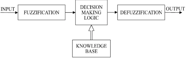
Figure 2.8: Fuzzy Controller Block Diagram

This classical logic, therefore, deals with combinations of variables that

The main content of classical logic is the study of rules that allow new logical

variables to be produced as functions of certain existing variables. Suppose that n logical

variables, x₁, x₂,..., x_n,, are given, say

1

x is true; 2

x is false;

. .

n

x is false.

Then a new logical variable, y, can be defined by a rule as a function of , x₁...,x _n

that has a particular truth value (again, either true or false). One example of a rule is the following:

1 2

: x x ... x_n y .

Rule IF is true AND is false AND AND is false THEN is false

2.5.2 Parameters Identification in Fuzzy Modeling

In order to solve the system modeling problem, we have to determine thevfollowing five items by using the available input-output data:

i. x₁,...,x_n: input variables, used as the premises of fuzzy logic implications.

ii. X₁,...,X_n: input variable intervals, used as fuzzy subsets.

iii. 1

X

µ ,...,

n X

µ : membership functions of the input variables, used to measure the qualities and quantities of the inputs.

In Step (i), generally speaking, to choose input variables x₁,...,x_n, first select

In Step (ii), all the input variable intervals are determined by estimating the ranges of the input values, or taking the minimum and maximum values of input variables directly from the data.

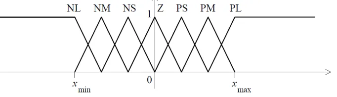
In Step (iii), all the membership functions of input variables are selected, more or less subjectively, by the designer based on his experience and the meaning of these functions to the real physical system. Uniform shape(s) of membership functions are usually desirable for computational efficiency, simple memory, and easy analysis. The most common choices of simple and efficient membership functions are triangular, trapezoidal, Gaussian functions. Since all input variables assume real values in general, or can be identified by (or mapped to) real values, the uniform triangular membership functions describing negative large (NL), negative medium (NM), negative small (NS), zero (Z), positive small (PS), positive medium (PM), and positive large (PL), all in absolute values, as shown in Figure 2.9, are very effective for system input (and output) variables.

Figure 2.9: Triangular membership functions over value range [x_min,x_max] of an input variable x.

2.5.3 Fuzzification

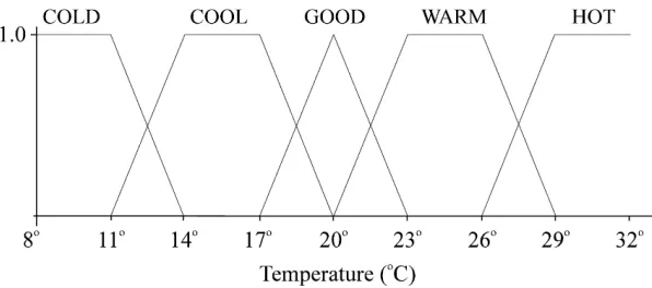
Figure 2.10: Fuzzy sets defining temperature

Each fuzzy set spans a region of input (or output) value graphed with the membership. Any particular input is interpreted from this fuzzy set and a degree of membership is interpreted. The membership functions should overlap to allow smooth mapping of the system. The process of fuzzification allows the system inputs and outputs to be expressed in linguistic terms so that rules can be applied in a simple manner to express a complex system.

Suppose a simplified implementation for an air-conditioning system with a temperature sensor. The temperature might be acquired by a microprocessor which has a fuzzy algorithm to process an output to continuously control the speed of a motor which keeps the room in a “good temperature,” it also can direct a vent upward or downward as necessary. The figure illustrates the process of fuzzification of the air temperature. There are five fuzzy sets for temperature: COLD, COOL, GOOD, WARM, and HOT.

The membership function for fuzzy sets COOL and WARM are trapezoidal, the membership function for GOOD is triangular, and the membership functions for COLD and HOT are halftriangular with shoulders indicating the physical limits for such process (staying in a place with a room temperature lower than 8 degrees Celsius or above 32 degrees Celsius would be quite uncomfortable).

2.5.4 Defuzzification

Defuzzification method is the final stage of the FLC. After the inference mechanism is finished. The defuzzification method tends converts the resulting fuzzy set into a crisp values that can be sent to the plant as a control signal.

In general, there are several methods used for defuzzification such as centroid of area (COA), maximum method (MM), mean of maximum (MOM), and bisector of area (BOA) [9]. The most frequently used are COA, MM, and MOM methods. First, MOM method produces the control action that represents the mean value of the all control actions whose membership function has the max value. Second is MM method that produces control action, which the fuzzy set reaches the maximum point. This method is divided into two parts: first, the smallest of max (SOM), which has the minimum value of the support of fuzzy set. The second method is the largest of max (LOM), which has the maximum value of the support of the fuzzy set.

The last is COA method that is used through this thesis. This method produces a control action that represents the center of the output of the fuzzy set. The weighted average of the membership function or the COA bounded by the membership function curve and it is converted to a typical crisp value. This method yield:

1

1 ( ).

( )

m

i i i

m

i i

x x u

x =

= µ =

µ

∑

∑

(2.6)

CHAPTER 3

METHODOLOGY

NO

NO

NO Study the Literature Review

3 D Modeling 6 DOF Robot in SolidWork (CAD)

Transfer 6 DOF Model to MATLAB/SIMULINK Desired Design

Tuning PID controller

Desired Result

Design a Fuzzy Logic controller

Desired Result

Finish Simulation

Simulation

YES

REFERENCES

1. M.W. Spong, S. Hutchinson and M. Vidyasagar, Robot Modeling and Control, 1st Edition, Jon Wiley & Sons, Inc, 2005.

2. J. Angeles, Fundamentals of Robotic Mechanical Systems: Theory, Methods, and

Algorithms, 2nd Edition, Springer, 2003.

3. Elena Garcia, Maria Antonia Jimenez, Pablo Gonzalez De Santos, And Manuel Armada The Evolution of Robotics Research, IEEE Robotics & Automation Magazine,

March 2007.

4. J.J. Crage, Introduction to Robotics Mechanics and Control, 3rd Edition, Prentice Hall, 2005.

5. K.J. Astrom and T. Hagglund, PID Controllers: Theory, Design and Tuning, 2nd Edition, Research Triangle Park, NC: Instrument Society of America, 1995.

6. Rocco, P., "Stability of PID control for industrial robot arms," Robotics and Automation,

IEEE Transactions on , vol.12, no.4, pp.606,614, Aug 1996

7. G.K.I. Mann, B.-G. Hu, and R.G. Gosine, “Analysis of Direct Action Fuzzy PID

Controller Structures,” IEEE Transactions on Systems, Man, and Cybernetics,Part B, Vol. 29, No. 3, pp. 371–388, Jun. 1999.

8. Z.-Y. Zhao, M. Tomizuka and S. Isaka, “Fuzzy Gain Scheduling PID Controller,”

IEEE Transactions on Systems, Man., Cybernetics Society, Vol. 23, No. 5, pp.1392–

1398, Sep/Oct. 1993.

9. G.M. Khoury, M. Saad, H.Y. Kanaan and C. Asmar, “Fuzzy PID Control of aFive

DOF Robot Arm,” Journal of Intelligent and Robotic systems., Vol. 40, No.3, pp.299–320, 2004.

10. Jie-Tong Zou ; Des-Hun Tu “The development of six D.O.F. robot arm for intelligent robot,” Control Conference (ASCC), 2011 8th Asian, pp. 976 – 981, 2011.

11. S. Elgazzar, “Efficient Kinematic Transformations for the Puma 560 Robot,”IEEE

Journal of Robotics and Automation., Vol. 1, No. 3, pp. 142–151, 1985.

12. A.C. Soh, E.A. Alwi, R.Z. Abdul Rahman and L.H. Fey, “Effect of Fuzzy Logic

University Journal of Science, Engineering and Technology., Vol. I,No. V, pp 28–39,

Sep. 2008.

13. A. Visioli, “Tuning of PID Controllers with Fuzzy Logic,” IEEE ProceedingsControl

Theory and Applications., Vol. 148, No. 1, pp. 1-8, 2001.

14. D.P. Kwok, Z.Q. Sun and P. Wang, “Linguistic PID Controller for Robot Arms,”IEEE

International Conference, Vol. 1, pp. 341–346, Mar. 1991.

15. S.G. Anavatti, S.A. Salman and J.Y. Choi, “Fuzzy + PID Controller for Robot

Manipulator,” International Conference on Computational Intelligence forModelling

Control and Automation., pp. 75, Dec. 2006.

16. G.K.I. Mann, B.-G. Hu, and R.G. Gosine, “Analysis of Direct Action Fuzzy PID Controller Structures,” IEEE Transactions on Systems, Man, and Cybernetics,Part B,

Vol. 29, No. 3, pp. 371–388, Jun. 1999.

17. Alassar A.Z., Abuhadrous I.M., Elaydi H.A., "Comparison between FLC and PID Controller for 5 DOF robot arm," Advanced Computer Control (ICACC), 2010 2nd

International Conference on , vol.5, no., pp.277,281, 27-29 March 2010.

18. J.G. Ziegler and N.B. Nichols, “Optimum Settings for Automatic Controllers,”

Transaction American Society of Mechanical Engineering., Vol. 64, pp. 759–768,

1942.

19. S. Annand, Software for Control and Dynamic Simulation of Unimate Puma 560

Robot, MS Thesis, The Faculty of the College of Engineering and Technology,

Ohio University, June 1993.

20. D.P. Kwok, Z.Q. Sun and P. Wang, “Linguistic PID Controller for Robot Arms,”