Variational Background Modeling Using Grid Point Sampling for Document Image Binarization

International Journal of Emerging Technology and Advanced Engineering

460

Variational Background Modeling Using Grid Point

Sampling for Document Image Binarization

J. Bharathi

_{, Dr. P. Chandrasekar Reddy}

1_{Associate Professor, Department of ECE, Deccan College of Engineering and Technology, Hyderabad} 2_{Professor, Department of ECE, JNTU College of Engineering, Hyderabad}

Abstract— Historical and degraded documents have varying background due to poor and uneven illumination, ageing of paper etc. Global thresholding methods give poor binarization results for these documents. Local binarization methods which are adaptive give enhanced results. Many image binarization algorithms and techniques are proposed in the literature. In this paper a new binarization technique is proposed and is compared with few standard techniques. The varying background is modeled based on the observation that the text pixels constitute less compared to the background pixels in document images. This technique is faster due to fewer computations and shows improved binarized image compared to standard adaptive binarization methods.

Keywords— Degraded documents, Document background estimation, Image binarization, Varying background illumination.

I. INTRODUCTION

An Optical Character Recognition (OCR) system typically has pre-processing, recognition and post processing modules. Pre-processing module acquires the images, removes skew and binarizes the image for further processing by the recognition module. Binarization is an important step in the document image processing and Optical Character Recognition systems. Old document images are difficult to binarize due to smear, uneven illumination, image contrast variation, bleeding of ink, etc. Poor binarization results in broken and touching characters which considerably affect the OCR performance. Therefore better binarization leads to better OCR recognition rates. In this paper an attempt is made to improve the binarization of degraded documents to get better OCR results. As the overall performance of an OCR system depends on the performance of individual modules, an improvement in any module increases the overall OCR performance [1].

Many thresholding techniques are proposed in the literature [2], [3], [4], [5]. These methods generally fall into two main categories namely global methods and local adaptive methods. Global methods apply a calculated threshold value to the entire image.

A simple way to automatically select a global threshold is to use the value at the valley of the intensity histogram of the image, assuming that there are two peaks in the histogram, one corresponding to the foreground, the other to the background. Local adaptive binarization methods, compute a threshold for each pixel in the image on the basis of information contained in a neighborhood. The local values are based on an assumed local neighborhood window. These algorithms perform better in certain types of documents and may give unsatisfactory results in other document. Hybrid methods combine both local and global information to find the pixel value [6].

A moment preserving method is proposed in [7]. In this the threshold is selected in such a way that the gray level moments of input image are preserved after binarization also. A minimum error thresholding based on statistical decision theory is presented in [8]. Low grade document binarization with bad illumination is investigated in [9], [10], [11], [12] and camera image binarization algorithm is proposed in [13].

In this paper we examine some of the important methods; their performances on the test document set and compare them with the proposed algorithm.

The paper is organized as follows: Thresholding methods are discussed in section II, Methodology of proposed method in section III, Experiments and results in section IV and conclusions in section V.

II. THRESHOLDING METHODS

Some of the widely used thresholding methods are discussed below.

A. Global Methods

International Journal of Emerging Technology and Advanced Engineering

461 Otsu proved that minimization of inter-class variance is the same as maximizing intra-class variance. The optimum threshold can be found automatically using the above maximization algorithm.

B. Local Adaptive Methods

Niblack Method: The idea of this method is to vary the threshold over the image, based on the local mean and local standard deviation [15]. The threshold at pixel (x,y) is calculated as T(x,y) = m(x,y) + k .s(x,y ) where m(x,y) and

s(x,y) are the sample mean and standard deviation values, respectively, in a local neighborhood of (x,y).The size of the neighborhood should be small enough to preserve local details, but at the same time large enough to suppress noise. We found a 15 x 15 neighborhood to be a good choice. The value of k is used to adjust how much of the total print object boundary is taken as a part of the given object; k = -0.2 gives well-separated print objects.

Bernsen Method: In this method, for each pixel (x, y), the threshold T(x, y) = ( Zlow + Zhigh )/2 is used, where Zlow and Zhigh are the lowest and highest gray level pixel values in a square [r x r] neighborhood centered at (x, y) [16]. However, if the contrast measure C(x, y) = (Zhigh – Zlow) <

L, where L is a constant, then the neighborhood consists only of one class, print or background. In our images, wide print areas rarely occur, so the pixel is labeled background in such cases. Trier and Jain [2] found L = 15 and r = 15 to be good choices.

Mean-Gradient Technique: A further improved variant of Niblack’s local thresholding approach, based on local mean and local mean-gradient values is proposed in this technique [4].

The gradient of the intensity image I(x,y) is:

∇I(x,y) = [∂I(x,y)/ ∂x, ∂I(x,y)/ ∂y]

The mean-gradient of the intensity image I(x,y) is:

G = ΣΣ [∂I(x,y)/ ∂x, ∂I(x,y)/ ∂y]/xy

The gradient is sensitive to noise, so the technique is improved by adding a pre-condition in selecting a threshold level: if Constant >= R

T(x, y) = M(x,y) + k G(x,y) else

T(x, y) = 0.5M(x,y)

where k = -1.5, R = 40; parameters M(x,y) and G(x,y) are the local mean and local mean-gradient calculated in a window centered at (x,y), Constant = Maximum grey value – minimum grey value in a window. If Constant > R, there will be high variance in the local window so that the mean-gradient value can correctly describe the characteristic of the local area.

Sauvola method: Sauvola et al [17] proposed this method. In this two algorithms are proposed to determine a local threshold for each pixel. A hybrid switch differentiates text, line drawings from background graphics. Non textual components are thresholded using soft decision based method and text components are thresholded using the equation T(x,y) = m(x,y).[1+ k

.((s(x,y) / R)-1)] where m(x,y) and s(x,y) are the same in Niblack’s method. R is the dynamic range of standard deviation and k is given positive values. R = 128 and k = 0.5 are suggested for 8-bit grey level image for good results.

Our Method (Grid Point Method): In the image documents the background has very large number of pixels compared to the foreground. The gray levels may be viewed as random variables in the range [0 1] for the images [18]. If we sample the image pixels we are more likely to get the background pixels rather than the foreground. About 50 documents are studied and all of them have shown small percentage of text pixels in histograms as in Fig. 1. This observation combined with median filter is used to model the back ground surface.

International Journal of Emerging Technology and Advanced Engineering

462 III. METHODOLOGY

A. Preprocessing

Old documents usually contain texture in back ground. Smoothing of the texture is essential to improve

Fig.2 Block diagram of the proposed method

binarization. Gaussian low pass filter is used to smoothen the image.

B. Grid Point Sampling

The binarization method is essentially a separation technique of foreground and background pixels. A grid of an arbitrary width and height is overlaid on the image. At the intersection points of grid the intensities of pixels are sampled. As the text in the document image contributes fewer pixels compared to the background, it is more probable that the pixels sampled belong to the background. It is observed in our experiments that only few foreground pixels are sampled. Figure 4 shows the sampled values as an image. The text values sampled at the grid intersection are removed by the suitable median filter. These sample values after applying the median filter as an image is shown Figure 5. The intensities at grid points are interpolated to obtain background intensity surface [Figure 6]. The background surface is the surface passing through points after applying the median filter and interpolation. The bi-cubic interpolation technique is used for the interpolation which gives smoother values at sampled points. Figure 7 shows a scan line of image and estimated background surface.

Fig.3 Scanned document image

Fig.4 Sampled background

Fig.5 Sampled background after applying median filter

Fig.6 Estimated background after applying median filter and interpolation

Fig.7 Intensities along a scan line (blue), estimated background (green) and threshold line (red)

C. Thresholding

The threshold surface T(x,y) is so chosen as to remove the noise and small variations occurred due to median filtering and pixel intensity interpolation in the estimated background by multiplying a suitable factor k [Fig. 7].

where k is a constant between 0-1 and is estimated background surface. Suitable k values are 0.8 – 0.9. Low values of k eliminate the noise but result in broken characters.

Preprocessing

I Sampling at

Grid Points

Thresholding

Removing print by median filter

IBF

International Journal of Emerging Technology and Advanced Engineering

463 The above surface T is used to binarize the filtered image.

where F is Foreground surface, p is pixel value, T is threshold value.

D. Automatic calculation of optimal k value

The thresholding surface can be viewed as a non-linear decision boundary surface which classifies or segments into pixels belonging to foreground and back ground. The number of pixels on each surface T defined as above gives histogram of corrected image for the varying illumination. This histogram will be bimodal as the varying background is modeled as non-linear surface and thresholding surface is a multiple of this. Optimally k

should be so chosen as to divide the above histogram at valley [Fig. 8].

Fig. 8 Graph between k and number of pixels np. The k at valley point is the optimal k value ko

The search for optimal k is started at kupper reducing k at an interval a. At each k, the number of pixels in a region

R, defined as a region between thresholding surfaces Tk and Tk+∆ are counted where ∆ is a small incremental value. By assigning suitable values for a and ∆ we can obtain smooth curve between k and number of pixels np. The k

corresponding to the lowest np is adopted as optimal value

ko. The algorithm is as follows:

1.

k = kupper – i*a, i = 0,1,2,… until k ≤ klower 3. Calculate the number of pixels np in the region R

4. Find the ko such that np is minimum

ko = argmin{np}

kupper = 0.98, a = 0.03 and ∆ = 0.02 are considered for calculation ko on the test data set.

Fig. 9 Algorithm for optimal ko

E. Post processing

The binarized image may still contain left over random noise spread across the image. This is especially true in the documents where bleeding phenomena is large. Here the noise is assumed to have isolated inverted pixel value either in the background or in the text as these pixels hardly constitute the background or text.

In the first stage, the image is scanned to identify the noise locations [Fig. 10]. A small window is placed at each location to identify the noise and moved along the entire image. In the second stage these pixel values are substituted with the surrounding pixel values. This scheme closes the opening in the text and eliminated random one pixel noise.

(a) (b)

Fig.10 (a) Single pixel noise in the background (b) Single pixel noise (Hole) in the text

The complete algorithm is as follows:

1. Read the document image and convert it into a grey scale image

International Journal of Emerging Technology and Advanced Engineering

464

3. Overlay a grid having arbitrary width and height over the image

4. Sample the pixel intensities at grid points to approximate the surface s

gs = grid size

Ng =Number of grid points along x Mg =Number of grid points along y

5. Apply median filter to remove the foreground pixels

6. Interpolate the intensities for the image size to estimate the background surface S(x,y)

7. Calculate the optimal k value, ko using algorithm in Fig. 9

8. Calculate the threshold surface T(x,y)

Where ko = optimal threshold value 9. Binarize the image with the threshold value T

10. Fill up holes and remove single pixel noise

N = Noise defined as

Fig.11 Algorithm for Grid Point method

(a)

(b)

(c)

(d)

International Journal of Emerging Technology and Advanced Engineering

465 (f)

(g)

Fig.12 (a) Original image (b) Otsu binarized (c) Niblack binarized (d) Bernsen binarized (e) Sauvola binarized (f) Mean gradient

binarized (g) Grid points binarized

(a)

(b)

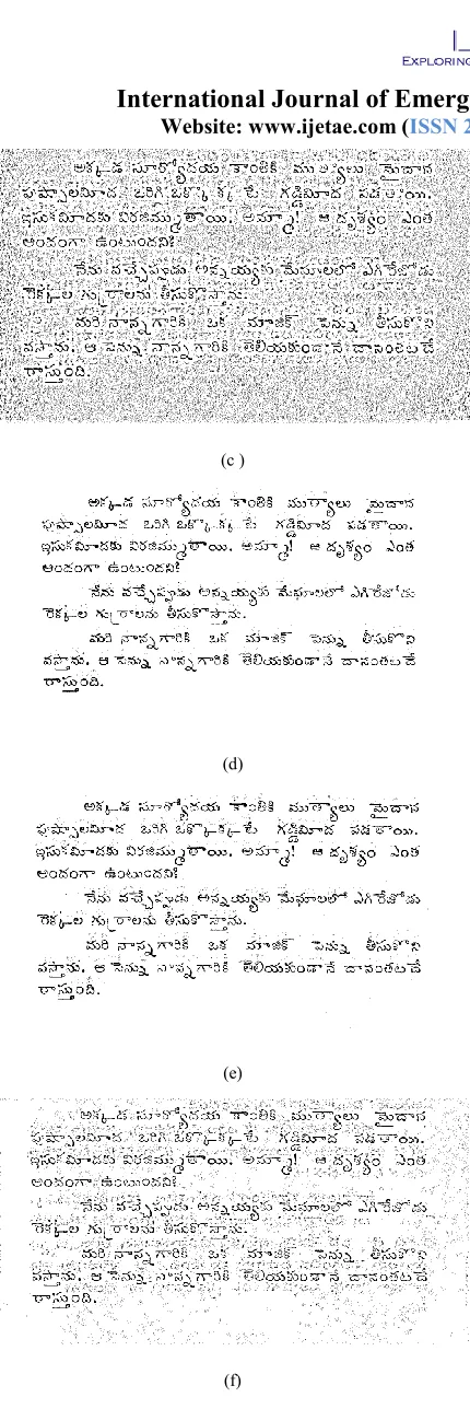
(c )

(d)

(e)

(f)

(g)

Fig.13 (a) Original image (b) Otsu binarized (c) Niblack binarized (d) Bernsen binarized (e) Sauvola binarized (f) Mean gradient

binarized (g) Grid points binarized

(a)

International Journal of Emerging Technology and Advanced Engineering

466 (c )

(d)

(e)

(f)

(g)

Fig.14 (a) Original image (b) Otsu binarized (c) Niblack binarized (d) Bernsen binarized (e) Sauvola binarized (f) Mean gradient

binarized (g) Grid points binarized

TABLE I

RESULTS

Method Otsu

Nib-lack Ber-nsen

Sau-vola

Mean gra-dient

Grid point

Fig. No. 12 12 12 12 12 12

PSNR 10.78 9.34 10.71 10.56 10.23 10.78

Precision 98.87 55.33 99.26 99.27 91.69 98.52

Recall 81.07 55.19 71.57 61.71 54.08 82.36

FM 89.09 55.26 83.17 76.11 68.03 89.72

Fig. No. 13 13 13 13 13 13

PSNR 10.02 9.66 12.21 12.19 11.90 11.81

Precision 24.90 35.25 89.46 99.01 87.72 97.48

Recall 66.47 40.52 31.98 35.35 37.96 69.47

FM 36.23 37.70 47.12 52.10 52.99 81.13

Fig. No. 14 14 14 14 14 14

PSNR 18.41 10.85 18.47 18.41 15.30 18.44

Precision 96.62 32.84 97.83 95.72 64.29 97.09

Recall 67.49 60.50 64.57 64.41 57.90 67.57

FM 79.47 42.58 77.79 77.00 60.93 79.68

IV. EXPERIMENTS AND RESULTS

International Journal of Emerging Technology and Advanced Engineering

467 Three sets of ten images each are taken from the three telugu books, one printed in 1925 (Srimadaandhra Mahabharathamu, Santhi Parvamu), another in 1966 (Translated works of Rabindranath Tagore) and the last a decade ago (a children’s book).

The proposed algorithm is compared with some of the known Global methods (Otsu) and Local adaptive methods (Niblack, Bernsen, Mean gradient, Sauvola). A window size of 15 x 15 with k = -0.2 are considered for Niblack method. For Sauvola method R=128 k = 0.5 are used. For Bernsen a window of 15x15 and contrast value of 15 are used. For mean gradient method k = -1.5 and contrast threshold level R = 40 are used.

A. Evaluation metrics

The performance evaluation is done as described in [19], [11]. The True Positive (TP), False Positive (FP) and False Negative (FN) pixels are counted with reference to the Ground Truth image to calculate Recall and Precision metrics.

A pixel is classified as TP if it is ON in both Ground Truth (GT) and binarization result images. A pixel is classified as FP if it is ON only in the binarization result image. A pixel is classified as FN if it is ON only in the GT image.

The Recall metric shows the ratio of the number of pixels, which a method truly classifies as foreground, to the number of all foreground pixels in the ground truth image.

Precision metric is the ratio of the number of pixels, which a method truly classifies as foreground, to the number of all pixels classified as foreground.

Denoting CTP as the number of TP pixels, CFP as the number of FP pixels and CFN as the number of FN pixels, Recall (RC) and Precision (PR) metrics are calculated as follows:

Recall and precision metric have values between zero and one and they are shown as percentages. As these metrics approach one (100%), the results get better. The overall metric that is used for evaluation is the FMeasure (FM) which is calculated as follows:

This measure evaluates how well an algorithm can retrieve the desired pixels.

Where

C is a constant that denotes the difference between foreground and background. This is considered as 255 for the 8-bit gray scale image. The PSNR measures how close the resultant image is to another. Therefore, the higher value of PSNR indicates more similarity between the two images.

B. Results

PSNR value is calculated between all the gray scale images and binarized images. The average PSNR value of 13.347 is achieved for the Grid Point method on the test set. The results amply demonstrate the efficiency of the proposed methodology for the degraded documents. In most of the cases it outperformed the other methods. Precision, recall and fm are calculated for comparing the results between Ground Truth images and binarized images [Table 1]. Ground Truth images are prepared only for three sample images.

The Ground Truth images are prepared by following the procedure described here. Initially the edges for the gray scale images are found by using the canny edge operator. Then the edges are meticulously verified for continuity and manually connected at appropriate locations to get the full continuous edges. The gap between the double edges is filled and the other unwanted specks are removed to get the final Ground Truth image.

International Journal of Emerging Technology and Advanced Engineering

468

V. CONCLUSIONS

In this paper, we proposed a fast and novel algorithm for binarization of degraded and variational background text image documents which leads to better OCR performance. The algorithm performed better than the Otsu, Niblack, Bernsen, Mean gradient method and Sauvola method for the test documents considered. Even though Telugu language documents are considered as images, this can be successfully applied to any other text images.

REFERENCES

[1] Pavan Kumar, P., Bhagvathi, C., Atul Negi, Agarwal, A. 2011. ―Towards Improving the Accuracy of Telugu OCR Systems‖, ICDAR ’11, pp. 910-914.

[2] Pal, N. R., Pal, S. K. 1993. ―A review on image segmentation‖, Pattern Recognition, Vol. 26, No. 9, , pp. 1277-1294.

[3] Trier, O. D., Jain, A. K., 1995. ―Goal-directed evaluation of binarization methods‖, IEEE Tran. Pattern Analysis and Machine Intelligence, PAMI-17, pp. 1191-1201.

[4] Leedham, G., Yan, C., Takru, K., Tan, J. H. N., Mian, L. 2003. ―Comparison of some thresholding algorithms for text/background segmentation in difficult document images‖, International Conference on Document Analysis and Recognition, pp. 859–864.

[5] Sankur, B., Sezgin, M. 2004. ―Survey over Image Thresholding Techniques and Quantitative Performance Evaluation,‖ Journal of Electronic Imaging, pp. 146-165.

[6] Kuo, T., Lai, Y., Lo, Y. 2010. ―A novel image binarization method using hybrid thresholding,‖ IEEE International Conference on Multimedia & Expo (ICME), pp. 608–612.

[7] Tsai, W. H. 1985. "Moment-preserving thresholding: A new approach," Comput. Vision, Graphics, Image Processing, vol. 29, pp. 377-393.

[8] Kittler and Illingworth, J., 1986 "Minimum error thresholding," Pattern Recognition, vol. 19, pp. 41-47.

[9] Gatos, B., Pratikakis, I., Perantonis,S. J. 2006. ―Adaptive degraded document image binarization‖, Pattern Recognition, 39(3): 317-327.

[10]Lu, S. J., Tan, C. L. 2007. ―Binarization of Badly Illuminated Document Images through Shading Estimation and Compensation‖ ICDAR 2007, pp. 312-316.

[11]Su, B., Lu, S., Tan, C. L. 2010. ―Binarization of historical handwritten document images using local maximum and minimum filter,‖ International Workshop on Document Analysis Systems, June 2010, pp. 159–165.

[12]Lu, S, Su, B., Tan, C. L. 2010. ―Document image binarization using background estimation and stroke edges‖, IJDAR, Vol.13, no.4, December 2010, pp. 303-314.

[13]Seeger, M, Dance, C. 2001. ―Binarizing camera images for OCR‖, 6th Int'l Conf. on. Document Analysis and Recognition, pp. 54-58.

[14]Otsu, N. 1978. ―A threshold selection method from gray level histogram,‖ IEEE Transactions on System, Man, Cybernetics, vol. 19, January, pp. 62–66.

[15]Niblack, W. 1986. An Introduction to Digital Image Processing, Englewood Cliffs, N.J. Prentice Hall, pp.115-116.

[16]Bernsen J. 1986. ―Dynamic thresholding of grey-level images,‖ Proc. Eighth Int’l Conj Pattern Recognition, Paris, pp. 1,251-1,255.

[17]Sauvola, J., Pietikainen, M. 2000. ―Adaptive Document Image Binarization‖, Pattern Recognition, 33, pp. 225–236.

[18]Gonzalez, R. C., Woods, R. E. 2002. Digital Image Processing, 2nd edition, Pearson Education, pp. 92.