CONTROL AND OPTIMIZATION
Volume5, Number3, September2015 pp.251–266
A GRADIENT ALGORITHM FOR OPTIMAL CONTROL PROBLEMS WITH MODEL-REALITY DIFFERENCES
Sie Long Kek
Department of Mathematics and Statistics Universiti Tun Hussein Onn Malaysia
86400 Parit Raja, Malaysia
Mohd Ismail Abd Aziz
Department of Mathematical Sciences Universiti Teknologi Malaysia 81310 UTM, Skudai, Malaysia
Kok Lay Teo
Department of Mathematics and Statistics Curtin University of Technology
Perth, W.A. 6845, Australia
Abstract. In this paper, we propose a computational approach to solve a model-based optimal control problem. Our aim is to obtain the optimal so-lution of the nonlinear optimal control problem. Since the structures of both problems are different, only solving the model-based optimal control problem will not give the optimal solution of the nonlinear optimal control problem. In our approach, the adjusted parameters are added into the model used so as the differences between the real plant and the model can be measured. On this basis, an expanded optimal control problem is introduced, where sys-tem optimization and parameter estimation are integrated interactively. The Hamiltonian function, which adjoins the cost function, the state equation and the additional constraints, is defined. By applying the calculus of variation, a set of the necessary optimality conditions, which defines modified model-based optimal control problem, parameter estimation problem and computation of modifiers, is then derived. To obtain the optimal solution, the modified model-based optimal control problem is converted in a nonlinear programming prob-lem through the canonical formulation, where the gradient formulation can be made. During the iterative procedure, the control sequences are generated as the admissible control law of the model used, together with the corresponding state sequences. Consequently, the optimal solution is updated repeatedly by the adjusted parameters. At the end of iteration, the converged solution ap-proaches to the correct optimal solution of the original optimal control problem in spite of model-reality differences. For illustration, two examples are studied and the results show the efficiency of the approach proposed.
2010Mathematics Subject Classification. Primary: 93C05, 93C10; Secondary: 93B40.
Key words and phrases. Nonlinear optimal control, model-reality differences, gradient
algorithm, adjusted parameters, iterative solution.
The reviewing process of the paper was handled by Cedric Yiu as Guest Editor.
1. Introduction. Linear quadratic regulator (LQR) problem is a standard optimal control problem, where the cost functional is in quadratic criterion and the state dynamics is in a linear form. Solving this optimal control problem is simple and the corresponding optimal solution is guaranteed [2], [5], [15]. Further from this, the applications of the LQR problem have been widely explored; see for examples, [13], [14], [10], [18], [9]. However, the nonlinear state dynamics is always linearized before a decision control policy is determined to minimize the cost function. In this point of view, the adjustable parameters are introduced in the LQR model such that the differences between the real plant and the model used can be measured repeatedly. At the end of iteration, the iterative solution could converge to the correct optimal solution of the original optimal control problem, in spite of model-reality differences [11], [12], [1].
Usually, the sweep method is applied to construct the feedback control law in solving the LQR model-based optimal control problem [2], [5]. It is the same work as those done by [11], [12], [1]. In this paper, we propose an efficient computation approach to construct the control sequences for the optimal control problem with model-reality differences. On this basis, the model-based optimal control problem, which is added with the adjusted parameters, is solved iteratively. Our aim is to ob-tain the true optimal solution of the original optimal control problem via solving the model-based optimal control problem repeatedly. For doing so, the initial control sequences are defined from the LQR optimal control model. Then, the modified model-based optimal control problem is formulated as a nonlinear programming problem [15], [6], [3]. During each iteration step, the differences between the real plant and the model used are measured by the adjusted parameters. It follows that the value of the control sequences is updated through the gradient algorithm, where the mathematical optimization technique is applicable. Within a given tolerance, the iterative algorithm gives the correct optimal solution of the original optimal control problem despite model-reality differences. It is highly recommended that the gradient algorithm can make the way of solving optimal control problems with model-reality differences more flexible.
The rest of the paper is organized as follows. In Section 2, a general class of optimal control problem is described. In Section 3, a simplified model-based optimal control problem is discussed, where the adjusted parameters are added into the model used. It points out that the interactive between system optimization and parameter estimation gives a modified optimal control problem, which can be solved by the gradient algorithm. Consequently, an efficient iterative algorithm is resulted. In Section 4, two illustrative examples are demonstrated and the efficiency of the approach proposed is shown. Finally, some concluding remarks are made.
2. Problem Description. Consider a general class of optimal control problem given below:
min
u(k)J0(u) =ϕ(x(N), N) + N−1
X
k=0
L(x(k), u(k), k)
subject to (1)
x(k+ 1) =f(x(k), u(k), k)
where u(k) ∈ <m, k = 0,1, . . . , N −1, and x(k) ∈ <n, k = 0,1, . . . , N, are, respectively, control and state sequences, whereasf :<n× <m× < → <n represents the real plant, ϕ : <n × < → < is the terminal cost andL : <n× <m× < → < is the cost under summation. Here, J0 is the scalar cost function and the initial statex0 is a known vector. It is assumed that all functions in (1) are continuously differentiable with respect to their respective arguments.
This problem is regarded as the real optimal control problem, and is referred to as Problem (P). Notice that this problem is a complex problem, where the structure of the problem is in nonlinear manner. Solving this kind of the problem is compu-tationally demanding. In view of this, we propose to solve a simplified model-based optimal control problem iteratively in order to obtain the correct optimal solution of Problem (P). Let this simplified model-based optimal control problem, which is referred to as Problem (M), be given below.
min u(k)
J1(u) = 1 2x(N)
>S(N)x(N) +γ(N)
+ N−1
X
k=0 1 2(x(k)
>Qx(k) +u(k)>Ru(k)) +γ(k)
subject to (2)
x(k+ 1) =Ax(k) +Bu(k) +α(k)
x(0) =x0
where α(k) ∈ <n, k = 0,1, . . . , N −1, and γ(k) ∈ <, k = 0,1, . . . , N, are the adjustable parameters, while A is an n×n state transition matrix and B is an n×m contol coefficient matrix. J1 is the model cost function, S(N) and Q are n×npositive semi-definite matrices, andRis a m×mpositive definite matrix.
Notice that solving Problem (M) iteratively would give the true optimal solution of Problem (P). This could be done because of the adjustable parameters that introduced into the model are able to measure the differences between the real plant and the model used repeatedly. In such way, we aim at approximating the correct optimal solution of Problem (P) by solving Problem (M), in spite of model-reality differences.
3. Gradient Algorithm with Model-Reality Differences. Now, let us intro-duce an expanded optimal control problem, which is referred to as Problem (E), given below.
min u(k)
J2(u) = 1 2x(N)
>S(N)x(N) +γ(N)
+ N−1
X
k=0 1 2(x(k)
>Qx(k) +u(k)>Ru(k)) +γ(k)
+1
2r1ku(k)−v(k)k 2+1
2r2kx(k)−z(k)k 2
subject to (3)
x(k+ 1) =Ax(k) +Bu(k) +α(k)
x(0) =x0 1 2z(N)
1 2(z(k)
>Qz(k) +v(k)>Rv(k)) +γ(k) =L(z(k), v(k), k)
Az(k) +Bv(k) +α(k) =f(z(k), v(k), k)
v(k) =u(k)
z(k) =x(k)
wherev(k)∈ <m,k= 0,1, . . . , N−1, andz(k)∈ <n,k= 0,1, . . . , N, are introduced to separate the control sequence and the state sequence in the optimization problem from the respective signals in the parameter estimation problem, andk · kdenotes the usual Euclidean norm. The terms 12r1ku(k)−v(k)k2and 12r2kx(k)−z(k)k2 with r1 ∈ < and r2 ∈ < are introduced to improve convexity and to facilitate convergence of the resulting iterative algorithm. It is important to note that the algorithm is designed such that the constraints v(k) = u(k) and z(k) = x(k) are satisfied upon termination of the iterations, assuming that convergence is achieved. The state constraintz(k) and the control constraintv(k) are used for the compu-tation of the parameter estimation and matching schemes, while the corresponding state constraint x(k) and control constraint u(k) are reserved for optimizing the model-based optimal control problem. In this way, system optimization and the parameter estimation are mutually interactive.
3.1. Necessary optimality conditions. Consider that the Hamiltonian function for Problem (E) is defined by
H2(k) =1 2(x(k)
>Qx(k) +u(k)>Ru(k)) +γ(k)
+1
2r1ku(k)−v(k)k 2+1
2r2kx(k)−z(k)k 2 +p(k+ 1)>(Ax(k) +Bu(k) +α(k))
−λ(k)>u(k)−β(k)>x(k) (4)
where λ(k) ∈ <m, k = 0,1, . . . , N −1, and β(k) ∈ <n, k = 0,1, . . . , N −1, are modifiers. Then, the augmented cost function becomes
J20(k) = 1 2x(N)
>S(N)x(N) +γ(N) +p(0)>x(0)−p(N)>x(N)
+ξ(N)(ϕ(z(N), N)−1
2x(N)
>S(N)x(N)−γ(N))
+Γ>(x(N)−z(N))
+ N−1
X
k=0
H2(k)−p(k)>x(k) +λ(k)>v(k) +β(k)>z(k)
+ξ(k)(L(z(k), v(k), k)−1
2(z(k)
>Qz(k) +v(k)>Rv(k))−γ(k))
+µ(k)>(f(z(k), v(k), k)−Az(k)−Bv(k)−α(k)) (5)
wherep(k), γ(k), ξ(k), µ(k),Γ, λ(k), andβ(k), are the appropriate multipliers to be determined later.
Applying the calculus of variation [2], [5], the following necessary optimality conditions are obtained.
(a) Stationary condition:
(b) Co-state equation:
p(k) =Qx(k) +A>p(k+ 1)−β(k) +r2(x(k)−z(k)) (6b) (c) State equation:
x(k+ 1) =Ax(k) +Bu(k) +α(k) (6c)
(d) Boundary conditions:
p(N) =S(N)x(N) + Γ andx(0) =x0 (6d)
(e) Adjustable parameter equations:
ϕ(z(N), N) =1 2z(N)
>S(N)z(N) +γ(N) (7a)
L(z(k), v(k), k) =1 2(z(k)
>Qz(k) +v(k)>Rv(k)) +γ(k) (7b)
f(z(k), v(k), k) =Az(k) +Bv(k) +α(k) (7c)
(f) Multiplier equations:
Γ =∇z(k)ϕ−S(N)z(N) (8a)
λ(k) =−(∇v(k)L−Rv(k))−
∂f
∂v(k)−B
>
ˆ
p(k+ 1) (8b)
β(k) =−(∇z(k)L−Qz(k))−
∂f ∂z(k)−A
>
ˆ
p(k+ 1) (8c)
withξ(k) = 1 andµ(k) = ˆp(k+ 1). (g) Separable variables:
z(k) =x(k), v(k) =u(k),p(k) =ˆ p(k) (9)
Notice that the parameter estimation problem is defined by (7) and the multipli-ers can be calculated from (8). Equations (6a) C (6d) are the necessary conditions for the modified model-based optimal control problem.
3.2. Modified optimal control problem. The modified model-based optimal control problem, which is referred to as Problem (MM), is given below.
min u(k)
J3(u) =1 2x(N)
>S(N)x(N) + Γ>x(N) +γ(N)
+ N−1
X
k=0 1 2(x(k)
>Qx(k) +u(k)>Ru(k)) +γ(k)
+1
2r1ku(k)−v(k)k 2+1
2r2kx(k)−z(k)k 2
−λ(k)>u(k)−β(k)>x(k)
subject to (10)
x(k+ 1) =Ax(k) +Bu(k) +α(k)
x(0) =x0
Once the state sequences are determined corresponding to the control sequences which can be defined through the gradient formulation, Problem (MM) could be converted in a nonlinear programming problem as given below [15], [6], [7], [8], [17]:
min u(k)
J3(u) subject tou(k)∈ <m, k= 0,1, . . . , N−1. Let this problem be Problem (MM’).
3.3. Admissible control law. Define
V ={v= [v1, . . . , vm]> ∈ <m:ai≤vi ≤bi, i= 1, . . . , m} (11)
where ai, i = 1, . . . , m, and bi, i = 1, . . . , m, are given real numbers. Notice that V is compact and convex subset of <m. Let u denote a control sequence
{u(k) :k= 0,1, . . . , N−1}inV. Then,uis called an admissible control. LetU be the class of all such admissible controls.
For each u∈ U, letx(k|u), k= 0,1, . . . , N, be a sequence in<n such that the difference equations with the initial condition as mentioned in Problem (MM) are satisfied. This discrete function is called the solution of the system in Problem (MM) corresponding tou∈U.
Let the control vectorube perturbed byεˆu, whereε >0 is a small real number and ˆuis an arbitrary but fixed perturbation ofugiven by
ˆ
u=(ˆu(0))>,(ˆu(1))>, . . . ,(ˆu(N−1))>>. (12)
This gives
uε=u+εˆu= [(u(0, ε))>,(u(1, ε))>, . . . ,(u(N−1, ε))>]> (13)
where
u(k, ε) =u(k) +εˆu(k), k= 0,1, . . . , N −1. (14)
Following from (14), the state of the model used in Problem (MM) will be perturbed, and so is the cost functionalJ3.
3.4. Gradient formula. Define the state sequences
x(k, ε) =x(k|ε), k= 1,2, . . . , N. (15)
Then, the system of difference equations in Problem (MM) becomes
x(k+ 1, ε) =Ax(k, ε) +Bu(k, ε) +α(k). (16)
The variation of the state (16) fork= 0,1, . . . , N−1, is
∆x(k+ 1) =dx(k+ 1, ε)
dε |ε=0=A∆x(k, ε) +Bu(k)ˆ (17a) with
∆x(0) = 0 (17b)
For the cost functional, it is considered that
∂J3(u)
∂u uˆ= limε→0
J3(uε)−J3(u)
ε ≡
dJ3(uε) dε |ε=0 = (S(N)x(N) + Γ)>∆x(N)
+ N−1
X
k=0
(Ru(k) +r1(u(k)−v(k))−λ(k))>uˆ
Consider the Hamiltonian function defined by (4) and the corresponding necessary conditions (6a) -C (6b), we obtain
∂J3(u)
∂u uˆ=(S(N)x(N) + Γ)
>∆x(N)
+ N−1
X
k=0
∂H
2(k)
∂u −p(k+ 1)
>B)ˆu(k) + (p(k)−p(k+ 1)>A
∆x(k)
Then, it follows from (17a) that
∂J3
∂uuˆ=(S(N)x(N) + Γ)
>∆x(N)
+ N−1
X
k=0
p(k)>∆x(k)−p(k+ 1)>∆x(k+ 1) +∂H2(k)
∂u uˆ (19)
Hence, from the boundary conditions (6d) and (17b), it yields that
∂J3(u) ∂u uˆ=
∂H2(0) ∂u(0) , . . . ,
∂H2(N−1) ∂u(N−1) ]
ˆ u.
Because of ˆuis arbitrary, we obtain the following gradient formula
∂J3(u)
∂u =
∂H2(0) ∂u(0) , . . . ,
∂H2(N−1) ∂u(N−1)
. (20)
We present this result in the following as a theorem [15], [6], [7], [8], [17].
Theorem 3.1. Consider Problem (MM’). The gradient of J3(u), where u= [(u(0))>,(u(1))>, . . . ,(u(N−1))>]>,
is given by (20).
3.5. Gradient algorithm. The computation of the gradient of the cost functional J3(u) is stated in the following algorithm.
Gradient algorithm
Data For a givenu= [(u(0))>,(u(1))>, . . . ,(u(N−1))>]>such that (11) is satisfied. Step 1 Solve the system of difference equations (6c) forward in time fromk= 0 to
k=N with initial condition (6d) to obtainx(k|u),k= 0,1, . . . , N.
Step 2 Solve the system of the co-state difference equations (6b) backward in time fromk=N tok= 1. Letp(k|u) be the solution obtained.
Step 3 Calculate the value of the cost functionalJ3(u) from (10). Step 4 Compute the gradient ofJ3(u) according to (20).
Remark: The gradient algorithm is used for updating the control sequence, solving the system of difference equations, to calculate the value of J3(u) and the corresponding gradient ofJ3(u) in Problem (MM’).
3.6. Iterative algorithm. From the discussion above, we shall summarize the result as an iterative algorithm, and the computation procedure is given below.
The iterative computation procedure
Step 0 Compute a nominal solution. Assuming thatα(k) = 0,k= 0,1, . . . , N−1, and r1 = r2 = 0. Solve Problem (M) defined by (2) to obtain u(k)0, k = 0,1, . . . , N −1, and x(k)0, p(k)0, k = 0,1, . . . , N. Then, with α(k) = 0, k = 0,1, . . . , N −1, and using r1, r2 from the data. Set i = 0, v(k)0 = u(k)0, z(k)0=x(k)0, and ˆp(k)0=p(k)0.
Step 1 Compute the parametersγ(k)i, k= 0,1, . . . , N, andα(k)i, k= 0,1, . . . , N− 1, from (7). This is called theparameter estimation step.
Step 2 Compute the modifiers Γi, λ(k)i and β(k)i, k = 0,1, . . . , N −1, from (8). Note that this step requires taking the derivatives off andLwith respect to v(k)i andz(k)i.
Step 3 Usingα(k)i, γ(k)i,Γi, λ(k)i, β(k)i, v(k)iandz(k)i, solve Problem (MM’) us-ing the result that is presented in Theorem 3.1 and the gradient algorithm. This is called thesystem optimization step.
3.1 Use (20) to obtain the new controlu(k)i, k= 0,1, . . . , N−1. 3.2 Use (6c) to obtain the new state ¯x(k)i, k= 0,1, . . . , N. 3.3 Use (6b) to obtain the new costatep(k)i, k= 0,1, . . . , N.
Step 4 Test the convergence and update the optimal solution of Problem (P). In order to provide a mechanism for regulating convergence, a simple relaxation method is employed:
v(k)i+1=v(k)i+kv(u(k)i−v(k)i) (21a)
z(k)i+1=z(k)i+kz(x(k)i−z(k)i) (21b)
ˆ
p(k)i+1= ˆp(k)i+kp(p(k)i−p(k)ˆ i) (21c)
where kv, kz, kp ∈ (0,1] are scalar gains. If v(k)i+1 = v(k)i, k = 0,1, . . ., N−1, andz(k)i+1 =z(k)i, k = 0,1, . . . , N, within a given tolerance, stop; else seti=i+ 1, and repeat the procedure starting with Step 1.
Remarks:
(a) A set of control sequences, which is for solving Problem (M) in Step 0, and for solving Problem (MM’) in Step 3, respectively, is determined from (20) by using the gradient algorithm.
(b) The parametersα(k)i, γ(k)i,Γi, λ(k)i, and β(k)i are zero in Step 0. Their calculated values, whereα(k)i andγ(k)iin Step 1, and Γi, λ(k)i, β(k)iin Step 2, change from iteration to iteration.
(c) Problem (P) is not necessary to be linear or to have a quadratic cost function. (d) The conditions v(k)i+1 = v(k)i and z(k)i+1 = z(k)i are required to be satisfied for the converged optimal control sequence and the converged state sequence, respectively. The following averaged 2-norms are computed, and then they are compared with a given tolerance to verify the convergence of v(k) andz(k):
kvi+1−vik2= 1 N−1
N−1
X
k=0
kv(k)i+1−v(k)ik !1/2
(22a)
kzi+1−zik2= 1 N
N
X
k=0
kz(k)i+1−z(k)ik !1/2
(22b)
may not result in an optimal number of iterations. It is important to note that the optimal choice of kv, kz, kp ∈ (0,1] is problem dependent, requiring that the proposed algorithm is run several times from Step 1 to Step 4. These values are initially set askv =kz=kp = 1 for the first run of the algorithm from Step 1 to Step 4, and then the algorithm is run with different values ranging from 0.1 to 0.9. The value that provides the optimal number of iterations can then be determined. The parametersr1 andr2are to enhance convexity, leading to the improvement of the convergence of the algorithm.
4. Illustrative Examples. Two illustrative examples are demonstrated here. They are continuous stirred-tank reactor problem [4] and inverted pendulum balancing problem [16].
Example 1: Consider a continuous stirred-tank reactor problem. The real plant is given by
x1(k+ 1) =x1(k)−0.02(x1(k) + 0.25) + 0.01(x2(k) + 0.5) exp
25x
1(k) x1(k) + 2
−0.01(x1(k) + 0.25)u(k)
x2(k+ 1) = 0.99x2(k)−0.005−0.01(x2(k) + 0.5) exp
25x1(k) x1(k) + 2
fork= 0,1, . . . ,77, with initial condition
x1(0) = 0.05, x2(0) = 0.
Our aim is to determine the control sequencesu(k),k= 0,1, . . . , N−1, so that the cost function
min u(k)
J0(u) = 0.01 N−1
X
k=0
(x1(k))2+ (x2(k))2+ 0.1(u(k))2
is minimized over the state dynamics.
This problem is referred to as Problem (P).
The simplified model-based optimal control problem, which is referred to as Prob-lem (M), is given below.
min
u(k)J1(u) = 1 2
N−1
X
k=0
[(x1(k))2+ (x2(k))2+ 0.1(u(k))2+ 2γ(k)] subject to
¯
x1(k+ 1) ¯
x2(k+ 1)
=
1.0895 0.0184
−0.1095 0.9716 ¯ x1(k) ¯ x2(k) + −0.003 0.000 u(k) +
α1(k) α2(k)
with the initial conditionx(0) = [0.05 0]>, and the adjusted parametersγ(k), and α(k) = [α1(k) α2(k)]>. The tolerance is set to 10−5.
0 0.1 0.2 0.3 0.4 0.5 0.6 0.7 0.8 −0.5
0 0.5 1 1.5 2
time, t
[image:10.612.156.446.136.363.2]control, u
Figure 1. Final control trajectoryu(k), Example 1
0 0.1 0.2 0.3 0.4 0.5 0.6 0.7 0.8
−0.04 −0.03 −0.02 −0.01 0 0.01 0.02 0.03 0.04 0.05
time, t
state, x
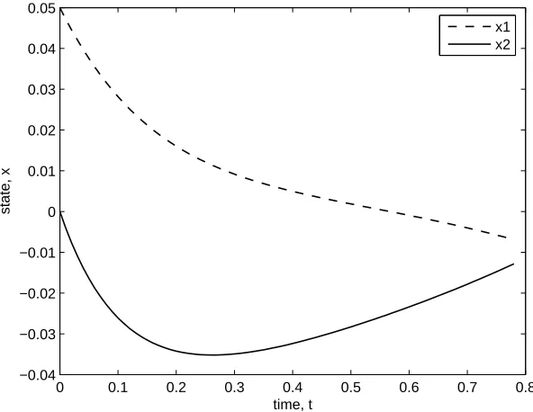
x1 x2
[image:10.612.150.446.420.649.2]0 0.1 0.2 0.3 0.4 0.5 0.6 0.7 0.8 −0.1
−0.05 0 0.05 0.1 0.15
time, t
alpha
[image:11.612.150.445.136.366.2]alp1 alp2
Figure 3. Adjusted parameterα(k), Example 1
0 0.1 0.2 0.3 0.4 0.5 0.6 0.7 0.8
−0.2 −0.15 −0.1 −0.05 0 0.05
time, t
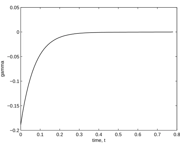
gamma
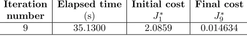
[image:11.612.149.447.412.651.2]Table 1. Simulation result, Example 1
Iteration Elapsed time Initial cost Final cost
number (s) J1∗ J9∗
9 35.1300 2.0859 0.014634
Example 2: Consider an inverted pendulum balancing problem. Problem (P) is described as follows. The state dynamic equations are discretized and given by
x1(k+ 1) =x1(k) + 0.1x2(k)
x2(k+ 1) =x2(k) +3.234 sinx1(k)−0.015(x2(k))
2cosx1(k) sinx1(k)
2.2−0.15(cosx1(k))2 (23) + 0.3u(k) cosx1(k)
2.2−0.15(cosx1(k))2 fork= 0,1, . . . ,29, with initial condition
x1(0) = 1.0, x2(0) = 0.5.
We aim to determine a set of the control sequencesu(k),k= 0,1, . . . , N−1, such that the cost function
min
u(k)J0(u) = 0.05 N−1
X
k=0
(x1(k))2+ (x2(k))2+ (u(k))2
is to be minimized over the state dynamics. The corresponding Problem (M) is given below.
min
u(k)J1(u) = 0.05 N−1
X
k=0
[(x1(k))2+ (x2(k))2+ 0.1(u(k))2+ 2γ(k)] subject to
¯
x1(k+ 1) ¯
x2(k+ 1)
=
1 0.1 1.5776 1
¯ x1(k) ¯ x2(k)
+
0.0000 0.1463
u(k) +
α1(k) α2(k)
with the initial conditionx(0) = [1.0 0.5]>, and the adjusted parametersγ(k) and α(k) = [α1(k) α2(k)]>. The given tolerance is 10−3.
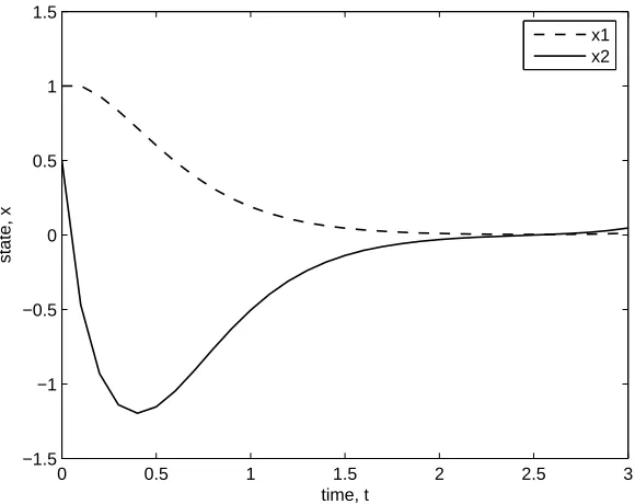
The simulation result is shown in Table 2 with the 79% efficiency of the algorithm proposed. Figures 5 and 6 show the trajectories of control and state, respectively, while Figures 7 and 8 show the adjusted parameters α(k) and γ(k), respectively. Since the values of the adjusted parameters tend to zero at the end of iteration step, it shows that the true optimal solution of the original optimal control problem is obtained despite model-reality differences.
Table 2. Simulation result, Example 2
Iteration Elapsed time Initial cost Final cost
number (s) J1∗ J7∗
[image:12.612.136.481.447.519.2]0 0.5 1 1.5 2 2.5 3 −35
−30 −25 −20 −15 −10 −5 0
time, t
[image:13.612.155.446.132.367.2]control, u
Figure 5. Final control trajectoryu(k), Example 2
0 0.5 1 1.5 2 2.5 3
−1.5 −1 −0.5 0 0.5 1 1.5
time, t
state, x
x1 x2
[image:13.612.155.445.419.649.2]0 0.5 1 1.5 2 2.5 3 −0.5
0 0.5 1 1.5 2
time, t
alpha
[image:14.612.154.446.132.368.2]alp1 alp2
Figure 7. Adjusted parameterα(k), Example 2
0 0.5 1 1.5 2 2.5 3
−450 −400 −350 −300 −250 −200 −150 −100 −50 0 50
time, t
gamma
[image:14.612.151.445.416.650.2]5. Concluding Remarks. A general class of discrete-time optimal control prob-lems, where model-reality differences is taken in account, was discussed in this paper. Because of the complexity of the original optimal control problem, a sim-plified model-based optimal control problem was proposed to be solved iteratively such that the true optimal solution of the original optimal control problem could be obtained. With introducing an expanded optimal control problem, we integrated system optimization and parameter estimation interactively. In addition to this, a modified optimal control problem was formulated as a nonlinear programming problem and it was solved by using the gradient approach. The resulting iterative algorithm, which integrates the gradient algorithm and the model-reality differ-ences, shows the efficiency through the illustrative examples discussed. On the other hand, the convergence of the adjusted parameters is guaranteed as Lipschitz condition is satisfied. In conclusion, the applicability of the algorithm proposed is highly recommended for solving nonlinear optimal control problems.
REFERENCES
[1] V. M. Becerra and P. D. Roberts,Dynamic integrated system optimization and parameter estimation for discrete time optimal control of nonlinear systems,Int. J. Control,63(1996), 257–281.
[2] A. E. Bryson and Y. C. Ho,Applied Optimal Control, Hemisphere Publishing Company, New York, 1975.
[3] S. L. Kek, Nonlinear programming approach for optimal control problems, Proceeding of the 2nd International Conference on Global Optimization and Its Applications, (2013), 20–25.
[4] D. E. Kirk, Optimal Control Theory: An Introduction, Mineola, NY: Dover Publications, 2004.
[5] F. L. Lewis and V. L. Syrmos,Optimal Control, 2nd ed, John Wiley & Sons, 1995.
[6] Q. Lin, R. Loxton and K. L. Teo,The control parameterization method for nonlinear optimal control: a survey,Journal of Industrial and Management Optimization,10(2014), 275–309. [7] R. Loxton, K. L. Teo and V. Rehbock,Computational method for a class of switched system optimal control problems,IEEE Transactions on Automatic Control,54(2009), 2455–2460.
[8] R. Loxton, K. L. Teo, V. Rehbock and K. F. C. Yiu, Optimal control problems with a continuous inequality constraint on the state and the control,Automatica,45(2009), 2250– 2257.
[9] L. F. Lupi´an and J. R. Rabad´an-Martin, LQR control methods for trajectory execution in omnidirectional mobile robots,Recent Advances in Mobile Robotics, (2011), 385–400.
[10] L. H. Nguyen, S. Park, A. Turnip and K. S. Hong, Application of LQR control theory to the design of modified skyhook control gains for semi-active suspension systems, Proceeding of ICROS-SICE International Joint Conference, (2009), 4698–4703.
[11] P. D. Roberts and T. W. C. Williams,On an algorithm for combined system optimization and parameter estimation,Automatica,17(1981), 199–209.
[12] P. D. Roberts, Optimal control of nonlinear systems with model-reality differences, Proceed-ings of the 31st IEEE Conference on Decision and Control,1(1992), 257–258.
[13] R. C. H. del Rosario and R. C. Smith, LQR control of shell vibrations via piezocreramic actuators, NASA Contractor Report 201673, ICASE Report No. 97-19, 1997.
[14] J. Saak and P. Benner, Application of LQR techniques to the adaptive control of quasilinear parabolic PDEs, Proceedings in Applied Mathematics and Mechanics, 2007.
[15] K. L. Teo, C. J. Goh and K. H. Wong,A Unified Computational Approach to Optimal Control
Problem, Longman Scientific and Technical, Essex, 1991.
[17] C. Z. Wu, K. L. Teo and V. Rehbock,Optimal control of piecewise affine systems with piece-wise affine state feedback,Journal of Industrial and Management Optimization, 5(2009), 737–747.
[18] B. Yang and B. Xiong, Application of LQR techniques to the anti-sway controller of overhead crane, Advanced Material Research,139-141(2010), 1933–1936.
Received May 2014; 1strevision June 2014; final revision March 2015.
E-mail address:[email protected]
E-mail address:[email protected]