Conditionbased maintenance modelling
Wang, W
Title
Conditionbased maintenance modelling
Authors
Wang, W
Type
Book Section
URL
This version is available at: http://usir.salford.ac.uk/2547/
Published Date
2008
USIR is a digital collection of the research output of the University of Salford. Where copyright
permits, full text material held in the repository is made freely available online and can be read,
downloaded and copied for noncommercial private study or research purposes. Please check the
manuscript for any further copyright restrictions.
Condition-based Maintenance Modelling
Wenbin Wang
5.1 Introduction
The use of condition monitoring techniques within industry to direct maintenance actions has increased rapidly over recent years to the extent that it has marked the beginning of what is likely to prove a new generation in production and maintenance management practice. There are both economic and technological reasons for this development driven by tight profit margins, high outage costs and an increase in plant complexity and automation. Technical advances in condition monitoring techniques have provided a means to achieve high availability and to reduce scheduled and unscheduled production shutdowns. In all cases, the measured condition information does, in addition to potentially improving decision making, have a value added role for a manager in that there is now a more objective means of explaining actions if challenged.
In November 1979, the consultants, Michael Neal & Associate Ltd published ‘A Guide to Condition Monitoring of Machinery’ for the UK Department of Trade and Industry, Neal et al (1997). This groundbreaking report illustrated the difference in maintenance strategies (e.g., breakdown, planned, etc.) and suggested that condition based maintenance, using a range of techniques, would offer significant benefits to industry. By the late 1990’s condition based maintenance had become widely accepted as one of the drivers to reduce maintenance costs and increase plant availability. With the advent of e-procurement, Business to Business (B2B), Customer to Business (C2B), Business to Customer (B2C) etc., industry is fast moving towards enterprise wide information systems associated with the internet. Today, plant asset management is the integration of computerised maintenance management systems and condition monitoring in order to fulfill the business objectives. This enables significant production benefits through objective maintenance prediction and scheduling. This positions the manufacturer to remain competitive in a dynamic market.
popular one for rotating and reciprocal machinery is the vibration analysis. However, irrespective of the particular condition monitoring technique used, the working principle of condition monitoring is the same namely, condition data becomes available which needs to be interpreted and appropriate actions taken accordingly. There are generally two stages in condition based maintenance. The first stage is related to condition monitoring data acquisition and its technical interpretations. There have been numerous papers contributing to this stage, as evidenced by the proceedings of COMADEM over recent years. This stage is characterised by engineering skill, knowledge and experience. Much effort of the study at this stage has gone into determining the appropriate variables to monitor, Chen et al (1994), the design of systems for condition monitoring data acquisition, Drake et al (1995), signal processing, Wong et al (2006), Samanta et al (2006), Harrison (1995), Li and Li (1995), and how to implement computerised condition monitoring, Meher-Homji et al (1994). These are just a few examples and no modelling is explicitly entered into the maintenance decision process based upon the results of condition monitoring. For detailed technical aspects of condition monitoring and fault diagnosis, see Collacott (1997). The second stage is maintenance decision making, namely what to do now given that condition information data and its interpretations are available. The decision at this stage can be complicated and entails consideration of cost, downtime, production demand, preventive maintenance shutdown windows, and most importantly, the likely survival time of the item monitored. Compared with the extensive literature on condition monitoring techniques and their applications, relatively little attention has been paid to the important problem of modelling appropriate decision making in condition based maintenance.
This chapter focuses on the second stage of condition monitoring, namely condition based maintenance modeling as an aid to effective decision making. In particular, we will highlight a modelling technique used recently in condition based maintenance, e.g. residual life modelling via stochastic filtering, Wang and Christer (2000). This is a key element in modeling the decision making aspect of condition based maintenance. The chapter is organised as follows. Section 5.2 gives a brief introduction to condition monitoring techniques. Section 5.3 focuses on condition based maintenance modeling and discuss various modeling techniques used. Section 5.4 presents the modelling of the residual life conditional on observed monitoring information using stochastic filtering. Section 5.5 concludes the chapter with a discussion of topics for future research.
5.2 Condition monitoring techniques
and/or temperature for an early indication of potential health problems, for industrial equipment some measurements can be taken and the likely condition of the plant assessed.
Today, there exists a large and growing variety of forms of condition monitoring techniques for machine condition monitoring and fault diagnosis. Understanding the nature of each monitoring technique and the type information measured will certainly help us when establishing a decision model. Here we briefly introduce five main techniques and among them, vibration and oil analysis techniques are the two most popular ones.
5.2.1 Vibration based monitoring
Vibration based monitoring is the main stream of current applications of condition monitoring in industry. Vibration based monitoring is an on (off) line technique used to detect system malfunction based on measured vibration signals.
Generally speaking, vibration is the variation with time of the magnitude of a quantity that is descriptive of the motion or position of a mechanical system, when the magnitude is alternatively greater than and smaller than some average value or reference.
Vibration monitoring consists of essentially in identifying two quantities:
- the magnitude (overall level) of the vibration - the frequency content (and/or time waveform)
The magnitude is basically used for establishing the severity of the vibration and the frequency content for the cause or origin. Vibration velocity has been seen as the most meaningful magnitude criterion for assessing machine condition, though displacement or acceleration is also used. The magnitude of vibration is usually measured in Root Mean Square (rms). If
T
denotes the period of vibration andV
(
t
)
is the vibration (say, velocity) measured at time t, then∫
=
T Trms
V
t
dt
V
0
2 1
(
(
))
,
which is proportional to the energy of vibration, Charles and Reeves (1998). However, since vibration signals from machines are, in general, periodic in nature, a great deal of information is contained in its frequency spectrum form. The frequency spectrum is usually obtained digitally using a digital analyser or computer via a mathematical algorithm known as “Fast Fourier Transform” (FFT). The spectrum analysis of vibration signals is commonly used in the fault diagnosis of rotating machines. Potentially, all machines can benefit from vibration monitoring except, perhaps, those running at very low speed (below about 20 rev/min), and those where isolation (or damping) occurs between the source and the sensor.
into play when establishing a vibration based maintenance model is the casual relationship between the measured signals and the state of the plant. It is the defect which causes the abnormal signals, but not vice versus, Wang (2002). This factor plays an important role when selecting an appropriate model for describing such a relationship.
5.2.2 Oil based monitoring
A detailed analysis of a sample of engine, transmission and hydraulic oils is a valuable preventive maintenance tool for machines. In many cases it enables the identification of potential problems before a major repair is necessary, has the potential to reduce the frequency of oil changes, and increase the resale value of used equipment.
Oil based monitoring involves sampling and analyzing oil for various properties and materials to monitor wear and contamination in an engine, transmission or hydraulic system etc. Sampling and analyzing on a regular basis establishes a baseline of normal wear and can help indicate when abnormal wear or contamination is occurring. Oil analysis works as follows. Oil that has been inside any moving mechanical apparatus for a period of time reflects the possible condition of that assembly. Oil is in contact with engine or mechanical components as wear metallic trace particles enter the oil. These particles are so small they remain in suspension. Many products of the combustion process also will become trapped in the circulating oil. The oil becomes a working history of the machine. Particles caused by normal wear and operation will mix with the oil. Any externally caused contamination also enters the oil. By identifying and measuring these impurities, one can get an indication of the rate of wear and of any excessive contamination. An oil analysis also will suggest methods to reduce accelerated wear and contamination.
The typical oil analysis tests for the presence of a number of different materials to determine sources of wear, find dirt and other contamination, and even check for the use of appropriate lubricants. Today there exist a variety of forms of oil based condition monitoring methods and techniques to check the volume and nature of foreign particles in oil for equipment health monitoring. There are spectrometric oil analysis, scan electron microscopy/energy dispersive x-ray analysis, energy dispersive x-ray fluorescent, low powered optical microscopy, and ferrous debris quantification. One purpose of the oil analysis is to provide a means of predicting possible impending failure without dismantling the equipment. One can "look inside" an engine, transmission or hydraulic systems without taking it apart.
difference when modeling the state of the plant in oil based monitoring compared to vibration based.
5.2.3 Other monitoring techniques
The other popular condition monitoring techniques are infrared thermography, accustics and the motor current analysis.
The basis of infrared thermography is quite simple. All objects emit heat or infrared electro-magnetic energy, but only a very small proportion of this energy is visible to a naked eye. At low temperatures in order to ‘see’ the heat being emitted an infrared camera must be used. The camera detects the invisible thermal energy and converts it to a visible image on a screen. The image can then be analyzed to identify any abnormality.
The acoustic emission (AE) based method is used widely for monitoring the condition of rotating machinery. Compared to traditional vibration based methods, the high frequency approach of AE has the advantage of a significant improvement in signal to noise ratio. It can also be used for non-rotating machinery where defect activities do not generate distinct repetition frequencies and hence FTT analysis cannot be used. An item to note is that AE transducers need to have a relatively narrow band to be able to detect high frequency faults.
The Motor current noise signature analysis methods and apparatus for monitoring the operating characteristics of an electric motor-operated device, such as a motor-operated valve, have been frequently used for early detection of rotor related faults in AC induction Motors. Frequency domain signal analysis techniques are applied to a conditioned motor current signal to distinctly identify various operating parameters of the motor driven device from the motor current signature. The signature may be recorded and compared with subsequent signatures to detect operating abnormalities and degradation of the device. This diagnostic method does not require special equipment to be installed on the motor-operated device, and the current sensing may be performed at remote control locations, e.g., where the motor-operated devices are used in unaccessible or hostile environments.
All the techniques briefly introduced above can offer some help for indicating the current state or condition of the plant monitored. Based on the technical analysis of the observed condition monitoring data, a maintenance decision has to be made to maintain the plant in a cost effective way. We discuss in the next section, how modeling can be used to support such a decision making utilizing available monitoring information.
5.3 Condition based maintenance modelling
optimise the maintenance to achieve minimum breakdown of the plant with maximum availability for production, and to ensure that maintenance is only carried out when necessary. This is what one calls condition based maintenance which contrasts with the traditional break down or time based maintenance policies where maintenance is only carried out when it becomes necessary utilizing available condition information. But in reality, all too often we see effort and money spent on monitoring equipment for faults which rarely occur, and we also see planned maintenance being carried out when the equipment is perfect healthy though the monitored information indicates something is ''wrong''. A study of oil based condition monitoring of gear boxes of locomotives used by Canadian Pacific Railway indicated, Aghjagan (1989), that since condition monitoring was commissioned (entailed 3-4 samples per locomotive per week, 52 weeks per year), the incidence failure of gear boxes while in use fell by 90%. This is a significant achievement. However, when subsequently stripped down for reconditioning/overhaul, there was nothing evidently wrong in 50% of cases. Clearly, condition monitoring can be highly effective, but may also be very inefficient at the same time. Modelling is necessary to improve the cost effectiveness and efficiency of condition monitoring.
5.3.1 The decision model
This is an extension to the age-based replacement model in that the replacement decision will be made not only dependent upon the age, but also upon the monitored information, plus other cost or downtime parameters. If we take the cost model as an example, then the decision model amounts to minimising the long run expected cost per unit time. We use the following notation:
f
c
: the mean cost per failure;p
c
: the mean cost per preventive replacement;m
c
: the mean cost per condition monitoring;i
t
: the ith and the current monitoring point;i
Y
: monitored information att
i withy
iof its observed value;i
ℑ
: history of observed condition variables tot
i,ℑ
i=
{
y
1,...,
y
i}
;i
X
: the residual life at timet
i;)
|
(
i i ix
p
ℑ
: pdf ofX
i conditional onℑ
i;The long term expected cost per unit time, , given that a preventive
replacement is scheduled at time t> is given by, Wang (2003),
)
(
t
C
i
t
0
(
) (
|
)
( )
(
)(1
(
|
))
i(
|
)
f p i i p m
t t
i i i i i i i i
c
c P t
t
c
ic
C t
t
t
t
P t
t
−x p x
dx
−
−
ℑ +
+
=
+ −
−
−
ℑ +
∫
ℑ
iwhere , which is the
probability of a failure before
t
conditiional on∫
−ℑ
=
ℑ
−
<
=
ℑ
−
t tii i i i i
i i i
i
P
X
t
t
p
x
dx
t
t
P
0
(
|
)
)
|
(
)
|
(
i
ℑ
. The right hand side of (5.1) is the expected cost per unit time formulated as a renewal reward function, though the life times are independent but not identical.The time point
t
is usually bounded within the time period from the current to the next monitoring since a new decision shall be made once a new monitoring reading becomes available at timet
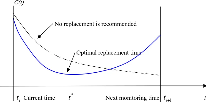
i+1.In general, if a minimum of is found within the interval to the next monitoring in terms of
t
, then thist
should be the optimal replacement time. If no minimum is found, then the recommendation would be to continue to use the plant and evaluate (5.1) at the next monitoring point when new information becomes available. For a graphical illustration of the above principle see Fig. 5.1.)
(
t
C
C(t)
No replacement is recommended
Optimal replacement time
t
i Current timet
* Next monitoring timet
i+1 t [image:8.595.127.458.344.514.2]
Fig. 5.1 A graph to show the optimal replacement time
Obviously the key element in (5.1) is the determination of
p
i(
x
i|
ℑ
i)
, which isthe topic of the next two sections,
5.3.2 Modelling
p
i(
x
i|
ℑ
i)
Before we proceed to the discussion of the modelling of
p
i(
x
i|
ℑ
i)
, there are few issues that need clarification.condition of the item monitored in a stochastic manner. For example in the vibration monitoring case, if a high vibration signal is observed we may suspect the item’s condition might be bad, but we may neither know the exact condition of it, nor its quantification. For direct monitored systems, Markov models are popular, see Black et al (2005), Chen and Trivedi (2005), and Love (2000). Counting processes have also been used for modeling the deterioration of directly monitored plant, see Aven (1996), Jenson (1992). Christer and Wang (1992) used a random coefficient model for a direct monitored case. It is noted however that the majority of condition monitoring applications are indirect monitoring such as the five popular monitoring techniques discussed earlier. It is therefore, in this chapter that our attention is paid to the indirect monitoring cases.
The second issue is the appropriate definition of the plant state. This also relates to the first issue whether the monitoring is direct or indirect. In direct monitoring, the actual observed condition of the item is clearly the plant state. While in the indirect monitoring case we can only observe measures indirectly related to the actual condition of the item monitored as discussed earlier. The most simple and intuitive definition is a set of categorical states ranging, say from 0 (new) to N (failed) as seen from Markov based models, Baruah and Chinnam (2005). Wang (2006a) also used a generic term of wear to represent the state of the monitored plant, which is particularly useful in modeling wear related problems in condition monitoring. Wang and Christer (2000) first used the residual life at the time of checking as a measure of the state of the monitored unit of interest. This definition provides an immediate modeling means to directly establish a link between the measured information and the residual life of interest. It is noted however, that this residual life is usually not observable which increases modeling complexity. A model of
p
i(
x
i|
ℑ
i)
introduced later will be based on thisdefinition.
Various different methods or models have been proposed in literature to formulate and calculate
p
i(
x
i|
ℑ
i)
. Proportional Hazard Modeling (PHM, one particular and natural form for modelling the hazard) is a popular one, Kumar and Westberg (1997), Love and Guo 1991, Makis and Jardine (1991), Jardine et al(1998), Banjevic et al (2001). Accelerated life models, Kalbfleisch and Prentice (1980), Wang and Zhang (2005) could also be used here, and may be more appropriate since the analogy between accelerated life testing, where these models originate, and condition monitoring is a close one. It should be noted that accelerated life models and proportional hazard models are identical when the time to failure distribution is Weibull, that is when the hazard function is given by
1
)
(
t
=
αβ
t
β−h
.via a covariate function. Both problems relate to the modeling assumption rather than the technique. The first one can be overcome if some sort of transformation of the observed data is used. The second problem remains unless the nature of monitoring indicates so. It is noted however that for most condition monitoring techniques, the observed monitoring measurements are concomitant types of information which are a function of the underlying plant state. A typical example is in vibration monitoring where a high level of vibration is usually caused by a hidden defect but not vice versus as we have discussed earlier. In this case the observed vibration signals may be regarded as concomitant variables which are caused by the plant state. Note that in oil based monitoring things are different as the metal particles and other contaminants observed in the oil can be regarded both as concomitant variables and covariates as we discussed earlier. In this case a model considers both variables might be appropriate.
The last decade has seen an increased use of stochastic filtering and Hidden Markov Models (HMM) for modelling
p
i(
x
i|
ℑ
i)
in condition based maintenance, Hontelez et al (1996), Christer et al (1997), Wang and Christer (2000), Bunka et al (2000), Dong and He (2004), Lin and Markis (2003, 2004), Baruah and Chinnam (2005), Wang (2006a). These techniques overcome both problems of PHM and provide a flexible way to model the relationship between the observed signals and unobserved plant state. HMM can be seen as a specific type of stochastic filtering models that are usually used for discrete state and observation variables. If the noise factors in the model are not Gaussian, then a closed form for is generally not available and one has to resort to numerical approximations. A comparison study using both filtering, Wang (2002), and PHM, Markic and Jardine (1991), based on vibration data revealed that the filtering based model produced a better result in terms of prediction accuracy, Matthew and Wang (2006).)
|
(
i i ix
p
ℑ
It should be noted also that if the monitored variables also influence the state to some extent, then both HMM and PHM should be used to tackle the problem. Alternatively an interactive HMM can also be formulated where a bilateral relationship is assumed between the observed and unobserved. In the next section, we shall discuss in details a specific filtering model used for the derivation of
. This model is simple to use and is analytically tractable.
)
|
(
i i ix
p
ℑ
5.4 Conditional residual life prediction
First we define the true state of plant is the residual life conditional upon measured condition related information to date, such as, vibration, temperature, etc..
though in a typical stochastic fashion. In theory, we may have the following relationship;
Defect short residual life higher than normal signal may be observed.
If the severity of the defect is represented by the length of the residual life, the relationship between the residual life and observed condition related variables follows.
5.4.1 Conditional residual life prediction
The model is built based on the following assumptions.
1. Plant items are monitored regularly at discrete time points.
2 There are two periods in the plant life where the first period is the time length from new to the point when the item was first identified to be faulty, and the second period is the time interval from this point to failure if no maintenance intervention is carried out. The second period is often called the failure delay time. It is also assumed that these two periods are statistically independent with each other.
3. A threshold level is established to classify the item monitored to be in a potential faulty state if the condition information signal is above the level. Such a threshold level is usually determined by engineering experience or by a statistical analysis of measured condition related variables.
4. The conditional information obtained at time
t
, , during the failuredelay time is a random variable which depends on .
i
y
i ix
Assumptions 1 and 2 can often be observed in condition monitoring practice. Assumption 3 can be relaxed and a model which can both identify the starting point of the second stage and residual life prediction can be established, Wang (2006b). For now to keep the model simple we still use assumption 3. Assumption 4 was first proposed in Wang and Christer (2000), which states that the rapid increase in the observed condition information is partly due to the shortened residual life because of the hidden defect. However this relationship is contaminated with random noise. Assumption 4 is the fundamental principle underpinning our model. For a detailed discussion on assumption 4 see Wang and Christer (2000).
Because the interest in residual life prediction is over the failure delay time (assuming it exists) and the information collected over the normal working period may not be beneficial for the residual life prediction, we revise our notation on
t
as the ith and the current monitoring time since the item was suspected to be faulty but still operating (noted that the order starts from the moment when the item was first identified to be possibly faulty). This implies thatt
is the first monitoring point which may indicate that the second stage has started. However, some monitoring may not be able to display a two-stage process such as oil basedi
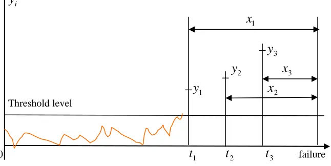
monitoring. If this is the case, we can simply set the threshold level to be zero. Fig. 5.2 shows a typical condition monitoring practice.
y
i
x
1y
3
y
2x
3
y
1x
2 Threshold level[image:12.595.135.458.203.365.2]
0
t
1t
2t
3 failureFig. 5.2 Condition monitoring practice
It is noted from Fig. 5.2 that the conditional information obtained before is not used since they are irrelevant to the decision making process. It is noted however, that the time to is one of important information sources to be used in determining the condition monitoring interval, Wang (2003).
1
t
1
t
Since the residual life at is the residual life at minus the interval
between and provided the item has survived to and no maintenance action has been taken, it follows that
i
t
t
i−1i
t
t
i−1t
i.
defined
if
)
(
1 1 11
⎩
⎨
⎧
−
−
>
−
=
− − − −else
not
t
t
X
t
t
X
X
i i i i i i i (5.2)The relationship between and is yet to be identified. From assumption 4 we
know that it can be described by a distribution, say, . We will discuss this later when fitting the model to data.
i
Y
X
i)
|
(
y
ix
ip
We wish to establish the expression of
p
i(
x
i|
ℑ
i)
, and therefore a consequential decision model can be constructed on the basis of such a conditional probability, see (5.1). Sinceℑ
i=
{
y
1,
y
2,...,
y
i}
=
{
y
i,
ℑ
i−1}
, thencan be expressed as
)
|
(
i i ix
p
ℑ
)
,
|
(
)
|
(
iℑ
i=
i iℑ
i−1i
x
p
x
y
(
) (
)
(
(
)
)
1 1 1|
|
,
,
|
|
− − −ℑ
ℑ
=
ℑ
=
ℑ
i i i i i i i i i i iy
p
y
x
p
y
x
p
x
p
(5.3)By using the multiplicative rule, the joint distribution,
p
(
x
i,
y
i|
ℑ
i−1)
is given as(
x
i,
y
i|
ℑ
i−1)
=
p
(
y
i|
x
i,
ℑ
i−1)
p
(
x
i|
ℑ
i−1)
p
(5.4)Since given both and , depends on only from assumption 4 so (5.4) reduces to
i
x
ℑ
i−1y
ix
i(
x
i,
y
i|
ℑ
i−1)
=
p
(
y
i|
x
i,
ℑ
i−1)
p
(
x
i|
ℑ
i−1)
=
p
(
y
i|
x
i)
p
(
x
i|
ℑ
i−1)
p
(5.5)Integrating out the
x
i term in (5.5) we havei i i i i i i i i i
i
p
x
y
dx
p
y
x
p
x
dx
y
p
ℑ
−=
∫
∞ℑ
−=
∫
∞ℑ
−0 1 0 1
1
)
(
,
|
)
(
|
)
(
|
)
|
(
(5.6)We focus our attention to
p
(
x
i|
ℑ
i−1)
which appears both in (5.4) and (5.6).From (5.2) we have
x
i−1=
g
(
x
i)
=
x
i+
(
t
i−
t
i−1)
conditional on. Then the distribution of 1
1 −
−
>
i−
ii
t
t
X
X
i|
ℑ
i−1 can be expressed by atransformation of variables from
X
i toX
i−1, Freund (2004), asi i i i i i i i i i
dx
x
dg
t
t
X
x
g
p
x
p
(
|
ℑ
−1)
=
−1(
(
)
|
ℑ
−1,
−1>
−
−1)
(
)
(5.7)Since
(
)
=
1
i i
dx
x
dg
and∫
∞− − − − − − − − − − − −ℑ
ℑ
=
−
>
ℑ
1 1 1 1 1 1 1 1 1 1 1)
|
(
)
|
)
(
(
)
,
|
)
(
(
i i tt i i i i
i i i i i i i i i
dx
x
p
x
g
p
t
t
X
x
g
p
(5.8)∫
∞− − − − − − − − − −ℑ
ℑ
−
+
=
ℑ
1 1 1 1 1 1 1 1 1)
|
(
)
|
(
)
|
(
i i tt i i i i
i i i i i i i
dx
x
p
t
t
x
p
x
p
(5.9)Using (5.5), (5.6) and (5.9), (5.3) becomes
(
)
(
)
1 1 1 0 1 1 1)
|
(
)
|
(
|
(
)
|
|
− − − ∞ − − −ℑ
−
+
ℑ
−
+
=
ℑ
∫
i i i i i i i ii i i i i i i i i i
dx
t
t
x
p
x
y
p
t
t
x
p
x
y
p
x
p
(5.10)(5.10) is a recursive equation which starts at time . At time , using (5.10) we have
1
t
t
1(
)
(
)
1 0 0 1 1 0 1 1 0 0 0 1 1 0 1 1 1 1 1)
|
(
)
|
(
|
(
)
|
|
dx
t
t
x
p
x
y
p
t
t
x
p
x
y
p
x
p
ℑ
−
+
ℑ
−
+
=
ℑ
∫
∞ (5.11)Since
ℑ
0 is usually 0 or not available, so)
(
)
|
(
1 1 0 0 0 1 1 00
x
t
t
p
x
t
t
p
+
−
ℑ
=
+
−
, then if and canbe specified, (5.11) can be determined. Similarly we can proceed to determining if and are available from the previous
step calculation at time .
)
(
00
x
p
p
(
y
1|
x
1)
)
|
(
i i ix
p
ℑ
p
i−1(
x
i−1|
ℑ
i−1)
p
(
y
i|
x
i)
1
−
i
t
Now the task is how to specify
p
0(
x
0)
andp
(
y
i|
x
i)
.5.4.2 Specification of
p
0(
x
0)
andp
(
y
i|
x
i)
.)
(
00
x
p
is just the delay time distribution over the second stage of the plant life. Here we use the Weibull dsitribution as an example in this context. In practice or theory, the distribution density function should be chosen from the one which best fits to the data or from some known theory.)
(
00
x
p
The set-up of the term requires more attention. Here we follow the
one used in Wang (2002), where is assumed to follow a Weibull
distribution with the scale parameter being equal to the inverse of . In this waywe establish a negative correlation between and as expected., that
is . The pdf is given below
)
|
(
y
ix
ip
i ix
y
|
i cxBe
A
+
−i
y
x
ii
cx i
i
i
X
x
A
Be
Y
η
η
η
( )1
)
(
)
|
(
cxii i i Be A y cx i cx i i
e
Be
A
y
Be
A
x
y
p
− − − − + −+
+
=
. (5.12)This is a concept called floating scale parameter, which is particularly useful in this case, Wang (2002). There are other choices to model the relationship between
and , but will not
i
y
i
x
be discussed here, and can be found in Wang (2006a).5.4.3 Estimating the model parameters within
p
i(
x
i|
ℑ
i)
To calculate the actual
p
i(
x
i|
ℑ
i)
we need to know the values for the modelparameters. They are the parameters of and . The most popular way to estimate them is using the method of maximum likelihood.
)
(
0 0x
p
p
(
y
i|
x
i)
At each monitoring point, , two pieces information are available, namely,
and , both conditional on
i
t
y
i1
1 −
−
>
i−
ii
t
t
X
ℑ
i−1. The pdf. fory
i|
ℑ
i−1 is given by (5.7) and the probability function ofX
i−1>
t
i−
t
i−1|
ℑ
i−1 is given by∫
∞− − − − − − − − −ℑ
=
ℑ
−
>
1 1 1 1 1 1 11
|
)
(
|
)
(
i i t
t i i i i
i i i
i
t
t
p
x
dx
X
P
(5.13)If the item monitored failed at time
t
f after the last monitoring at timet
n, the complete likelihood function is then given by)
|
(
)
)
|
(
)
|
(
)
(
1 1 1 1 1 1 1 n f n n
n
i
p
y
i i t tp
ix
i idx
ip
t
t
L
i iℑ
−
⎟
⎠
⎞
⎜
⎝
⎛
ℑ
ℑ
=
Θ
∏
=∫
∞− − − − −
−
−
(5.14)
where is the set of parameters to be estimated. Taking log on both sides of (5.14) and maximising it in terms of unknown parameters should give the estimated values of those parameters. However, computationally it has to be solved numerically since (5.14) involves many integrals which may not have analytical solutions.
Θ
5.4.4 A case study
typical stochastic nature of the life distribution. The monitored vibration signals also indicate an increasing trend with bearing ages in all cases, but with different paths. An important observation is the pattern of vibration signals which stays relatively flat in the early stage of the bearing life and then increases rapidly (a defect may have been initiated). This indicates the existence of the two stage failure process as defined earlier.
Fig. 5.3 Vibration data of six bearings
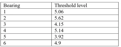
The initial point of the second stage in these bearings is identified using a control chart called the Shewhart average level chart and the threshold levels of the bearings are shown in table 5.1, Zhang (2004).
Table 5.1 Threshold level for each bearing
Bearing Threshold level
1 5.06 2 5.62 3 4.15 4 5.14 5 3.92 6 4.9
Assuming both distributions for
p
0(
x
0)
andp
(
y
i|
x
i)
are Weibull whereβ
α β
α
αβ
1 ( )0 0
0
)
(
)
(
x
x
e
xp
=
− − [image:16.595.184.415.497.587.2]η
η
η
( )1
)
(
)
|
(
cxii i i Be A y cx i cx i i
e
Be
A
y
Be
A
x
y
p
− − − − + −+
+
=
then starting from
t
1 and after recursive filtering we have∫
∞∏
∏
= + − − = + − −+
+
=
ℑ
0 1 )) ( ( 1 1 )) ( ( 1)
,
(
)
(
)
,
(
)
(
)
|
(
ik k i
t z i
i
k k i i
t x i i i i i
dz
t
z
e
t
z
t
x
e
t
x
x
p
i i iψ
ψ
β β α β α β (5.15) where ) ( ) ) (( ( ) 1
)
,
(
k i k t i t z C k t t z C Be A y i kBe
A
e
t
z
− + −+ −
+
=
− − + − ηψ
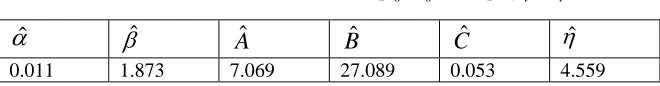
.To estimate the parameters in and we need write down the likelihood function as (5.14). The actual process to estimate these unknown parameters is complicated and involves heavy numerical manipulation which we omit and interested readers can get the details in Zhang (2004). The estimated result is listed in table 5.2.
)
(
00
x
[image:17.595.133.463.490.533.2]p
p
(
y
i|
x
i)
Table 5.2 Estimated parameter values in
p
0(
x
0)
andp
(
y
i|
x
i)
α
ˆ
β
ˆ
A
ˆ
B
ˆ
C
ˆ
η
ˆ
0.011 1.873 7.069 27.089 0.053 4.559
Fig. 5.4 Predicted condition residual life of bearing 6
In Fig.5.4 the actual residual lives at those checking points are also plotted with symbol *. It can be seen that actual residual lives are well within the predicted residual life distribution as expected.
Given the estimated values for parameters and associated costs such as
, and
6000
=
f
c
c
p=
2000
c
m=
30
, Wang and Jia (2001), we have the expected cost per unit time for one of the bearings at various checking time t, shown in Fig. 5.5.15 19 23 27
0 10 20 30
Planned replacement time
Expectd cost per unit time
t=80.5 hrs t=92.5 hrs t=104 hrs t=116.5 hrs t=129 hrs
[image:18.595.153.457.496.658.2]In can be seen from Fig. 5.5. that at t=116.5 and 129 hours both planned replacements are recommended within the next 30 hours.
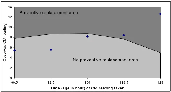
To illustrate an alternative decision chart in terms of the actual condition monitoring reading, we transformed the cost related decision into actual reading in Fig. 5.6 where the dark grey area indicates that if the reading falls within this area a preventive replacement is required within the planning period of consideration. The advantage of Fig. 5.6 is that it can not only tell us whether a preventive replacement is needed but also show us how far the reading is from the area of preventive replacement so that appropriate preparation can be done before the actual replacement.
0 2 4 6 8 10 12 14
80.5 92.5 104 116.5 129
Tim e (age in hour) of CM reading taken
Observed CM reading
Preventive replacem ent area
[image:19.595.146.442.290.449.2]No preventive replacem ent area
Fig. 5.6 Decision chart using observed CM reading.
The transformation is carried out in this way. At each monitoring point of , by
gradually changing the value of in
i
t
i
y
p
i(
x
i|
ℑ
i)
used in (5.1) until a preventive replacement is recommended by the model within the planning period, and then mark this value of as the threshold value at time . Connecting these threshold values at those monitoring points forms the boundary between the light and dark grey areas. Finally mark the actual reading of on the graph to see which area it falls in.i
y
t
ii
y
5.5
Future research directions
5.5.1 Multi-component systems
replacement such as bearings, pumps and motors, and various probability distributions are used to describe the life time of the component. In the case of a high value and high risk system with many components such as aircraft engines and gas turbines, how to assess the health condition and make prognosis based on condition information obtained from all components is still an open question. It is typical with a multi-component system that many observed signal parameters are available and the times between failures are neither independent nor identical.
5.5.2 Idebtification of the initial point of a random defect
With the delay time concept, see chapter 14, system life is assumed to be classified into two stages. The first is the normal working stage where no abnormal condition parameters are to be expected. The second starts when a hidden defect is first initiated with possible abnormal signals. The identification of the initial point in the evolution of such a defect is important and has a direct impact on the subsequent prediction model. Most research on fault diagnosis focuses on the location of the fault, the possible cause of the fault, and of course, the type of fault. This serves for the engineering purpose of deciding what to repair, but does not aid the decision of when to do the task. This initial point defect identification has received very little attention in prognosis literature. Wang (2006b) addressed this problem to some extent using a combination of the delay time concept and the HMM. Much work still remains. It is possible that a multi-stage (>2) failure process could be used, which might be more appropriate to some cases.
5.5.3 The definition of plant state
The definition of the underlying state and the relationship between the observed monitoring parameters and the state of the system are issues which still need attention. In the model presented in this chapter, the state of the system is defined as the residual life, which is assumed to influence the observed signal parameters. Whilst the modelling output appears to make sense, there are a few potential problems with the approach. The first is the issue that the life of the plant is fixed at birth (installation) but unknown. This is termed as playing the God. Secondly, the residual life is not the direct cause of the observed abnormal signals. These are more likely caused by some hidden defects which are linked to the residual life in this chapter. To correct the first problem we can introduce another equation describing the relationship between and deterministically or randomly.
This will allow to change during use, which is more appropriate. If the relationship is deterministic, then a closed form of (5.3) is still available, but if it is random, HMM must be used and no closed form of (5.3) exists unless the noises associated are normally distributed. The second problem can be overcome if we adopt a discrete or continuous state hidden Markov chain to describe the system deterioration process where the state space of the chain represents the system state under question.
i
X
X
i−1i
5.5.4 Information fusion
There is now a considerable amount of condition monitoring and process control information available in industry, thanks to the recent development in condition monitoring technology. It is noted that not all information are useful, or because of correlation they may provide similar information. There are two ways to deal with this. One is to use some statistical methods to reduce the dimension of the original data such as principal component analysis, and the other is to use multi-variate distributions. The principal component analysis method has been used in Wang and Zhang (2005), but unless the first principle component accounts for most of the variation in the original data we still need to deal with a data set with more than two dimensions. The use of multi-variate distributions in prognosis has not been reported apart from the normal distribution which has the drawback of producing negative values.
A final point worth mentioning is that in practice observed condition monitoring variables could be concomitant variables or covariates with respect to the system state. A model which can handle both type of information is ideal, but very few attempts have been made, Hussin and Wang (2006).
5.6 Summary and Conclusions
This chapter introduces the concept of condition monitoring, key condition monitoring techniques, condition based maintenance and associated modelling support in aid of condition based maintenance. Particular attention is paid to the residual time prediction based on available condition information to date. An important development made here is the establishment of the relationship between the observed information and underlying condition which is the residual life in this case. This is achieved by letting the mean of the observed information at be a
function of the residual life at that point conditional on
i
t
i
i
x
X
=
. The mathematical development is based on a recursive algorithm called filtering where all past information is included. The example illustrated is based on real data which came from a fatigue experiment. However, data from industry has showed the robustness of the approach and the residual life predictions conducted so far are satisfactory.5.6 References
Aghjagan, H.N., 1989, Lubeoil analysis expert system, Canadian Maintenance Engineering Conference, Toronto.
Aven T, 1996, Condition based replacement policies - a counting process approach, Rel. Eng. & Sys. Safety, 51(3), 275-281.
Baruah P., and Chinnam R.B., 2005, HMM for diagnostics and prognostics in maching processes, I. J. Prod. Res., 43(6), 1275-1293.
Black M., Brint, A.T., and Brailsford J.R., 2005, A semi-Markov approach for modelling asset deterioration, J. Opl. Res. Soc. 56(11), 1241-1249.
Bunks C., McCarthy D., and Al-Ani T., Condition based maintenance of machine using hidden Markov models, 2000, Mech. Sys. & Sig. Pro., 14(4), 597-612.
Charles W. Reeves, 1998, The vibration monitoring handbook, Coxmoor Publishing Company, Oxford, 1998.
Chen, W., Meher-Homji, C.B. and Mistree, F., 1994, COMPROMISE: an effective approach for condition-based maintenance management of gas turbines. Engineering Optimization, 22, 185-201.
Chen D. and Trivedi K.S., 2005, Optimization for condition based maintenance with semi-Markov decision process, Rel. Eng. & Sys. Safety, 90(1), 25-29.
Christer A.H and Wang W., 1995, A simple condition monitoring model for a direct monitoring process, E. J. Opl. Res., 82, 258-269.
Christer A.H. and Wang W., 1992, A model of condition monitoring inspection of production plant, I. J. Prod. Res., 30, 2199-2211.
Collacott, R.A., 1977, Mechanical fault diagnosis and condition monitoring, Chapman and Hall Ltd., London.
Dong M., and He D., 2004, Hidden semi-Markov models for machinery health diagnosis and prognosis, Trans. North Amer. Manu. Res. Ins. of SME, 32, 199-206.
Drake, P.R., Jennings, A.D., Grosvenor, R.I. and Whittleton, D., 1995, acquisition system for machine tool condition monitoring. Quality and Reliability Engineering International 11, 15-26.
Freud J.E., 2004, Mathematical statistics with applications, Pearson Prentice and Hall, London.
Harrison, N., 1995, Oil condition monitoring for the railway business. Insight 37, 278-283. Hontelez J.A.M., Burger H.H. and Wijnmalen D.J.D., 1996, Optimum condition based
maintenance policies for deteriorating systems with partial information, Rel. Eng. & Sys. Safety, 51(3), 267-274.
Hussin B, and Wang, W., 2006, Conditional residual time modelling using oil analysis: a mixed condition information using accumulated metal concentration and lubricant measurements, to appear in Proc. 1st Main. Eng. Conf, Chendu, China.
Jardine A.K.S., Makis V., Banjevic D., Braticevic D., and Ennis M., 1998, A decision optimization model for condition based maintenance, J. Qua. Main. Eng., 4(2), 115-121. Jensen U., 1992, Optimal replacement rules based on different information level, Naval Res.
Log. 39, 937-955.
Kalbfleisch, J.D. & Prentice, R.L., 1980, The Statistical Analysis of Failure Time Data. Wiley, New York.
Kumar, D., and Westberg U., 1997, Maintenance scheduling under age replacement policy using proportional hazard modelling and total-time-on-test plotting, Euro. J. Opl. Res.,
99, 507-515.
Li, C.J. & Li, S.Y., 1995, Acoustic emission analysis for bearing condition monitoring.
Wear 185, 67-74.
Lin D., and Makis V., 2003, Recursive filters for a partially observable system subject to random failures, Adv. Appl. Prob., 35(1), 207-227.
Lin D., and Makis V., 2003, Filters and parameter estimation for a partially observable system subject to random failures with continuous-range observations, , Adv. Appl. Prob., 36(4), 1212-1230.
Love, C.E. & Guo, R., 1991, Using proportional hazard modelling in plant maintenance.
Makis V. and Jardine A.K.S., 1991, Computation of optimal policies in replacement models,
IMA J. Maths. Appl. Business & Industry, 3, 169-176.
Matthew C., and Wang W., 2006, A comparison study of proportional hazard and stochastic filtering when applied to vibration based condition monitoring, submitted to Int. Tran OR.
Meher-Homji, C.B., Mistree, F. and Karandikar, S., 1994, An approach for the integration of condition monitoring and multi-objective optimization for gas turbine maintenance management. International Journal of Turbo and Jet Engines, 11, 43-51.
Neal M., and Associates, 1979, Guide to the condition monitoring of machinery, DTI, London.
Samanta, B., Al-Balushi, K.R., Al-Araimi, S.A. 2006, Artificial neural networks and genetic algorithm for bearing fault detection Soft Computing, 10 (3), 264-271. Wang W., 2002, A model to predict the residual life of rolling element bearings given
monitored condition monitoring information to date, IMA. J. Management Mathematics,
13, 3-16.
Wang W., 2003, Modelling condition monitoring intervals: A hybrid of simulation and analytical approaches, J. Opl. Res Soc, 54, 273-282.
Wang W., 2006a, A prognosis model for wear prediction based on oil based monitoring, to appear in J. Opl. Res Soc,
Wang W., 2006b, Modelling the probability assessment of the system state using available condition information, to appear in IMA. J. Management Mathematics.
Wang W. and A.H. Christer , 2000, Towards a general condition based maintenance model for a stochastic dynamic system, J. Opl. Res. Soc. 51, 145-155.
Wang W., and Jia, Y., 2001, A multiple condition information sources based maintenance model and associated prototype software development, proceedings of COMADEM 2001, Eds. A. Starr and Raj B.K.N. Rao, Elsevier, 889-898.
Wang W., and Zhang W., 2005, A model to predict the residual life of aircraft engines based on oil analysis data, Naval Logistics Research, 52, 276-284.
Wong, M.L.D., Jack, L.B., Nandi, A.K., 2006, Modified self-organising map for automated novelty detection applied to vibration signal monitoring Mech. Sys.
& Sig. Proc., 20(3), 593-610.
Zhan Y. Makis V., and Jardine A.K.S., 2006, Adaptive state detection of gearboxes under varying load conditions based on parametric modeling, Mech. Sys. & Sig. Prod. 20(1), 188-221.
Zhang W., 2004, Stochastic modeling and applications in condition based maintenance, PhD, thesis, University of Salford, UK.