BIROn - Birkbeck Institutional Research Online
Joseph, Agnell Praveen and Lagerstedt, I. and Patwardhan, A. and Topf,
Maya and Winn, M. (2017) Improved metrics for comparing structures of
macromolecular assemblies determined by 3D electron-microscopy. Journal
of Structural Biology 199 (1), pp. 12-26. ISSN 1047-8477.
Downloaded from:
Usage Guidelines:
Please refer to usage guidelines at
or alternatively
Improved metrics for comparing structures of macromolecular
assemblies determined by 3D electron-microscopy
Agnel Praveen Joseph
a,b, Ingvar Lagerstedt
c,d, Ardan Patwardhan
c, Maya Topf
a,⇑, Martyn Winn
b,⇑a
Institute of Structural and Molecular Biology, Department of Biological Sciences, Birkbeck College, University of London, Malet Street, London WC1E 7HX, United Kingdom b
Scientific Computing Department, Science and Technology Facilities Council, Research Complex at Harwell, Didcot OX11 0FA, United Kingdom c
European Molecular Biology Laboratory, European Bioinformatics Institute, Wellcome Genome Campus, Hinxton, Cambridge CB10 1SD, United Kingdom d
Computational Chemistry and Cheminformatics, Lilly UK, Windlesham GU20 6PH, United Kingdom
a r t i c l e i n f o
Article history:
Received 15 October 2016
Received in revised form 19 May 2017 Accepted 23 May 2017
Available online 25 May 2017
Keywords:
3D electron cryo-microscopy Integrative modelling Scoring functions Macromolecular assemblies Density fitting
a b s t r a c t
Recent developments in 3-dimensional electron microcopy (3D-EM) techniques and a concomitant drive to look at complex molecular structures, have led to a rapid increase in the amount of volume data avail-able for biomolecules. This creates a demand for better methods to analyse the data, including improved scores for comparison, classification and integration of data at different resolutions. To this end, we developed and evaluated a set of scoring functions that compare 3D-EM volumes. To test our scores we used a benchmark set of volume alignments derived from the Electron Microscopy Data Bank. We find that the performance of different scores vary with the map-type, resolution and the extent of overlap between volumes. Importantly, adding the overlap information to the local scoring functions can signif-icantly improve their precision and accuracy in a range of resolutions. A combined score involving the local mutual information and overlap (LMI_OV) performs best overall, irrespective of the map category, resolution or the extent of overlap, and we recommend this score for general use. The local mutual infor-mation score itself is found to be more discriminatory than cross-correlation coefficient for intermediate-to-low resolution maps or when the map size and density distribution differ significantly. For comparing map surfaces, we implemented two filters to detect the surface points, including one based on the ‘extent of surface exposure’. We show that scores that compare surfaces are useful at low resolutions and for maps with evident surface features. All the scores discussed are implemented in TEMPy (http://tempy. ismb.lon.ac.uk/).
Ó2017 The Authors. Published by Elsevier Inc. This is an open access article under the CC BY license (http:// creativecommons.org/licenses/by/4.0/).
1. Introduction
A major leap in structure characterization of large bio-molecular machines and cellular components has been brought in by biophysical techniques like electron microscopy (EM) and tomography (ET) (Bai et al., 2013; Kuhlbrandt, 2014; Milne et al., 2013), which result in 3D volume representations of the structure. The Electron Microscopy Data Bank (EMDB) (http://emdb-empiar. org) currently holds over 4000 volume reconstructions from EM and ET, and the number of entries has doubled in the last four years due to increasing interest and development of better image recon-struction methods and direct electron detectors (Kuhlbrandt, 2014).
Rapid increase in the amount of EM/ET data necessitates ways to categorize and compare them. Comparison of 3D-EM recon-structions (volume alignment) is useful to categorize existing data and annotate new volume depositions. Conformational changes involved in specific biological systems can also be studied by com-paring densities that represent different functional states.
The resolution of the 3D-EM data is often insufficient to provide atomic details of the macromolecular structure. Hence, atomic models of components are usually fitted into volumes to obtain an atomic representation of the structure (Villa and Lasker, 2014). Fitting atomic components into a target density is usually dealt with as a problem of volume alignment by first filtering the atomic model (probe) to the resolution of the target density before comparison (Chacon and Wriggers, 2002; Roseman, 2000; Rossmann, 2000; Topf and Sali, 2005; Volkmann and Hanein, 1999). Given an accurate placement derived from rigid-body align-ment (rigid fitting), further refinealign-ment of the model can be applied locally by sampling conformations that improve the fit with the
http://dx.doi.org/10.1016/j.jsb.2017.05.007
1047-8477/Ó2017 The Authors. Published by Elsevier Inc.
This is an open access article under the CC BY license (http://creativecommons.org/licenses/by/4.0/).
⇑Corresponding authors.
E-mail addresses: [email protected] (M. Topf), [email protected]
(M. Winn).
Contents lists available atScienceDirect
Journal of Structural Biology
target density (flexible fitting) (Topf et al., 2008; Trabuco et al., 2008; Wang and Schroder, 2012).
The available approaches for fitting or volume alignment are either using a map density based 6D grid search or a coarse-grained representation of volumes to reduce the search space. Exhaustive 6D search of the density grid does not suffer from den-sity approximations or coarse graining but is relatively slow. To reduce the computational cost, either the rotational search is accel-erated using spherical harmonics transforms (Garzon et al., 2007) or a Fast Fourier Transform (FFT) is employed to rapidly scan the translations (Chacón and Wriggers, 2002; Roseman, 2000; Wriggers, 2012). Random (Goddard et al., 2007) or stochastic sam-pling (Topf and Sali, 2005) of the search space can also reduce com-putation time but is more effective when the probe and target volumes do not have a large difference in size. Cross-correlation coefficient (CCC) between the search and target map densities is typically the metric used in these methods to optimize the fit.
Methods relying on coarse-grained representation of volumes are faster but the accuracy largely depends on the efficiency of fea-ture approximation. The molecular shape can be encoded with a set of feature points (Birmanns and Wriggers, 2007; Woetzel et al., 2011; Wriggers, 2012), even in the absence of interior den-sity features. A least square fit starting from triplet points from fea-ture sets (similar to geometric hashing) corresponding to probe and target, is performed to obtain the alignment. The sets of fea-ture points are then compared using RMSD metric and the fit opti-mized using CCC score. Another approach based on vector quantization, represented density maps as alpha shapes that approximates the map geometry and topology (De-Alarcón et al., 2002). Volume densities are also described using 3D Zernike moments (Esquivel-Rodriguez and Kihara, 2012) and the Euclidean distance of the coefficients is computed to calculate the similarity of two volumes. Common features or substructures can be also derived using rotationally invariant local density gradient descrip-tors (Saha and Morais, 2012; Saha et al., 2010). The histograms of these local density gradient vectors are matched to compare the local density and the alignment is performed by matching graphs that representing the feature points.
GMfit (Kawabata, 2008) relies upon a representation of the map density in terms of a Gaussian Mixture Model (GMM), which is a linear combination of a certain number of 3D anisotropic Gaussian Distribution Functions (GDFs). A score based on the overlap of two Gaussian mixtures is optimized to obtain the alignment. The num-ber of GDFs controls the description of the map; a larger numnum-ber generates a more detailed density function. There are several ways to obtain initial configurations in the 6D search to align two GMMs. These include random sampling, segmentation-based or symmet-ric fitting, or by matching principal axes, followed by a local steep-est descent optimization. The main computational cost is for the optimization of GDFs to generate the GMM while the comparison of Gaussian mixtures is usually carried out in seconds.
Apart from the alignment methodology, resolution, conforma-tional differences and the extent of noise in the density maps also influence the efficiency of volume comparisons. A major factor that determines the selection of correct orientations in the search space is the accuracy of metric used to score the alignments (Farabella et al., 2015; Henderson et al., 2012; Schneidman-Duhovny et al., 2012; Volkmann and Hanein, 1999). It becomes necessary to eval-uate and re-rank the proposed solutions using different scoring functions depending on the level of details in the volume recon-struction. Vasishtan and Topf (Vasishtan and Topf, 2011) presents an account of several scoring functions to evaluate the quality of alignment between two volumes, using either the density distribu-tion of the volume or the shape of the surface of the density distri-bution contoured at a certain value or both. TEMPy is a Python toolkit for volume and model processing and assessment in which
these scoring functions as well as additional ones are implemented (Farabella et al., 2015). Dugan and Altman assessed different scores for evaluating the match between a model and a surface envelope (Dugan and Altman, 2004). They proposed a metric favouring atom inclusion in the density while penalizing those lying outside the envelope. A similar score is used to evaluate fitted models associ-ated with 3D-EM data depositions in EMDB (Lagerstedt et al., 2013).
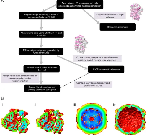
In the context of the BioMedBridges project (Field et al., 2013), we have developed a pipeline for comparison of volumes to catego-rize and annotate existing volume data (PDBeShape; to be pub-lished). The precision and accuracy of scoring functions has been a major bottleneck in the assessment of solutions proposed by dif-ferent volume comparison methods in this project. We therefore evaluated different scoring functions for their ability to distinguish correct volume alignments. We gathered a benchmark set of pair-wise alignments of experimental 3D-EM reconstructions from the EMDB, using superposition of associated fitted coordinate models to provide a ground truth fit. We used GMfit (Kawabata, 2008) as the volume alignment method as it is relatively fast and a poten-tially useful method for volume database searches. For each pair of volumes, the set of alignments generated by GMfit were scored using different metrics and the metrics were then evaluated based on the similarity of the alignments with the reference fit. We tested potential improvements and normalization of the scoring functions discussed in (Vasishtan and Topf, 2011). We could characterise dif-ferent scoring functions in terms of the class and resolution of the volumes involved, and the extent and nature of the overlap.
2. Methods
2.1. Dataset preparation
All 904 density maps (volumes) in the EMDB with correspond-ing fitted coordinate models in the PDB (as of April 2016) were considered. 50 maps each were chosen randomly from two major categories, ribosomes and viruses, and 30 maps for the categories of chaperones and other sample types; structure superposition of fitted atomic coordinates corresponding to maps in each category was carried out using MMalign (Mukherjee and Zhang, 2009) in order to define the ground truth alignments. For each alignment, MMalign calculates the TMscore which is a normalized score for evaluating the quality of superposition of atomic models, indepen-dent of the length of protein chains (Zhang and Skolnick, 2004, 2005). Alignments with TMscore >0.4 (Xu and Zhang, 2010) were chosen and the transformation leading to superposition was used to transform the corresponding maps with respect to each other. However, even when the TMscore was good, the alignment of cor-responding volumes could be non-optimal or incorrect due to fit-ting errors associated with one or both of the models and/or ambiguity in fitting at intermediate-low resolutions. We manually inspected the generated map-to-map alignments to remove those without correct matching orientations and selected a final refer-ence set of 28 alignments (ribosome: 7, virus: 8, chaperones: 6 and various: 7) covering different resolutions and map types (Table 1). Examples of a reference alignment from each of the major categories are shown inFig. S1. The 7 map-pairs not involv-ing ribosomes, viruses or chaperones, includes two gamma secre-tase, one TRPV1 channel, one ryanodine receptor, one ATPase (Type-V) and two RNA polymerase pairs. For our category-based analysis of alignments, we included these 7 additional map pairs together with the 6 chaperone pairs in the category ‘others’.
the number of Gaussians used to represent a volume, the more fea-tures can be abstracted and the better is the description of the den-sity. The number of Gaussians used to approximate a map was inferred from the number of segments found by Segger (Pintilie et al., 2010). Segger (implemented in Chimera (Pettersen et al., 2004)) is widely used for segmenting volumes to identify compo-nent shapes in the volume density. An initial application of the watershed algorithm is followed by iterative scale-space filtering and grouping resulting in larger and fewer segments.
In our implementation, we terminated the grouping when the observed number of segments falls below an expected number. We calculated the lower limit for the approximate number of seg-ments expected from the volume by estimating the theoretical protein volume corresponding to 100 amino acids (Harpaz et al., 1994) and scaling it by a factor of map resolution
SV¼ ð1001101:21Þ r ð1Þ
Here,SVis the effective volume of a segment in Å3, scaled by the resolutionr(in Å) of the map. 110 Da was used as the average molecular weight of each amino acid and 1.21 Å3/Da is the factor obtained by considering an average partial specific volume of
[image:4.595.37.553.104.362.2]0.73 cm3/g, for proteins. Dividing the total molecular volume by this scaled segment volume gives the number of segments expected, with the Segger procedure terminating at the next itera-tion at some number lower than this. The latter was then taken as the number of Gaussians to be used in GMfit. The theoretical vol-ume is scaled by the map resolutionrso that a lower resolution map is represented by fewer Gaussians compared to a higher res-olution map. In practice, we also imposed a minimum number of segments of 3 and a maximum number of 240. The selected num-ber of Gaussians for each volume in the test dataset is given in
Table 1. To match volumes abstracted by different Gaussian mix-tures, the random search protocol in GMfit was used, followed by a steepest descent local optimization (Kawabata, 2008).
As explained below, score calculations require assignment of an appropriate contour level for the volumes so that the density beyond this level can be considered as background noise. We determined contour density threshold based on the volume corre-sponding to the molecular weight of the macromolecule. For EMDB entries the molecular weights details provided by the authors may not be accurate or may not account for all components in the sample. Hence, we also considered the author-suggested contour level, and calculated the molecular volume from that. If the contour calculated from the estimated molecular weight falls below the background peak or above 5*sigma (where sigma is the standard deviation of density values, calculated with the back-ground peak as mean), then the author-suggested contour value is used instead. If the author-suggested level also fails the sanity check, then 1.5*sigma above the background peak is used. Also, if the contour level based on the molecular weight (as submitted to EMDB) differed significantly from the contour suggested by the authors (>3 sigma), the latter was used. The selected contour levels were manually verified. Next, we low-pass filtered the maps to the lower resolution of the two, using TEMPy (Farabella et al., 2015) and the grid spacing was set to 1/4 of that resolution (van Zundert et al., 2017). The transformation proposed by GMfit for each fit was applied to the maps, followed by the calculation of dif-ferent scores. The accuracies of difdif-ferent scoring functions (below) were then assessed using these proposed alignments with respect to the reference alignment. All the scores, band-pass filters and grid resampling functions are implemented in TEMPy (Farabella et al., 2015).
The following scores were selected based on their performance in previous tests on a simulated map dataset (Vasishtan and Topf, 2011) and the differences in the features they score, e.g. the voxel density values, binned densities, map surface features, surface den-sity gradients, extent of overlap etc. Potential modifications and improvements to these scores (see below) were also tested in this analysis.
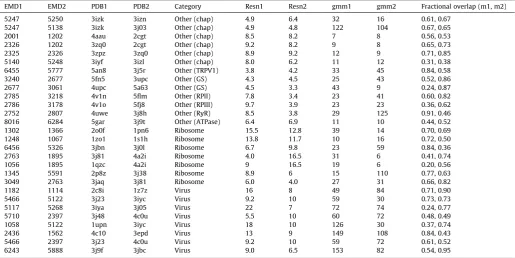
Table 1
Dataset used for evaluating scoring functions. The EMDB IDs of the volumes aligned, their associated fitted PDBs (PDB1 and PDB2), sample category, their resolutions (resn1 and resn2) and the number of Gaussian functions used for each map (gmm1 and gmm2), are given. The fraction of overlapping region from the reference map alignment with respect to the size of each map, is given in the last column. GS: Gamma secretase, RPII: RNA polymerase II, RPIII: RNA polymerase III, RyR: Ryanodine receptor.
EMD1 EMD2 PDB1 PDB2 Category Resn1 Resn2 gmm1 gmm2 Fractional overlap (m1, m2)
5247 5250 3izk 3izn Other (chap) 4.9 6.4 32 16 0.61, 0.67
5247 5138 3izk 3j03 Other (chap) 4.9 4.8 122 104 0.67, 0.65
2001 1202 4aau 2cgt Other (chap) 8.5 8.2 7 8 0.56, 0.53
2326 1202 3zq0 2cgt Other (chap) 9.2 8.2 9 8 0.65, 0.73
2325 2326 3zpz 3zq0 Other (chap) 8.9 9.2 12 9 0.71, 0.85
5140 5248 3iyf 3izl Other (chap) 8.0 6.2 11 12 0.31, 0.38
6455 5777 5an8 3j5r Other (TRPV1) 3.8 4.2 33 45 0.84, 0.58
3240 2677 5fn5 3upc Other (GS) 4.3 4.5 25 43 0.52, 0.86
2677 3061 4upc 5a63 Other (GS) 4.5 3.3 43 9 0.24, 0.87
2785 3218 4v1n 5flm Other (RPlI) 7.8 3.4 23 41 0.60, 0.82
2786 3178 4v1o 5fj8 Other (RPIII) 9.7 3.9 23 23 0.36, 0.62
2752 2807 4uwe 3j8h Other (RyR) 8.5 3.8 29 125 0.91, 0.46
8016 6284 5gar 3j9t Other (ATPase) 6.4 6.9 11 10 0.44, 0.52
1302 1366 2o0f 1pn6 Ribosome 15.5 12.8 39 14 0.70, 0.69
1248 1067 1zo1 1s1h Ribosome 13.8 11.7 10 16 0.72, 0.50
6456 5326 3jbn 3j0l Ribosome 6.7 9.8 23 59 0.84, 0.36
2763 1895 3j81 4a2i Ribosome 4.0 16.5 31 6 0.41, 0.74
1056 1895 1qzc 4a2i Ribosome 9 16.5 19 6 0.20, 0.56
1345 5591 2p8z 3j38 Ribosome 8.9 6 15 110 0.77, 0.63
3049 2763 3jaq 3j81 Ribosome 6.0 4.0 27 31 0.66, 0.82
1182 1114 2c8i 1z7z Virus 16 8 49 84 0.71, 0.90
5466 5122 3j23 3iyc Virus 9.2 10 59 30 0.73, 0.73
5117 5268 3iya 3j05 Virus 22 7 72 74 0.24, 0.77
5710 2397 3j48 4c0u Virus 5.5 10 60 72 0.48, 0.49
1058 5122 1upn 3iyc Virus 18 10 126 30 0.37, 0.74
2436 1562 4c10 3epd Virus 13 9 149 108 0.84, 0.43
5466 2397 3j23 4c0u Virus 9.2 10 59 72 0.61, 0.52
2.2. Density-based scores
The following scores consider the voxel density values for calcu-lations. Local score calculations are carried out over all voxels that are within the contour of both maps, i.e. the overlap region.
Theglobal Cross Correlation(CCC) was calculated as:
CCC¼
P
ðxxÞðyyÞ
ffiffiffiffiffiffiffiffiffiffiffiffiffiffiffiffiffiffiffiffiffiffiffi P
ðxxÞ2 q
qffiffiffiffiffiffiffiffiffiffiffiffiffiffiffiffiffiffiffiffiffiffiffiPðyyÞ2 ð2Þ
wherexand y are density values in each voxel in the two volumes being compared andxandyare the respective mean densities. The
Local Cross Correlation(SCCC) is calculated as:
SCCC¼
P
ðxxÞðyyÞ
ffiffiffiffiffiffiffiffiffiffiffiffiffiffiffiffiffiffiffiffiffiffiffi P
ðxxÞ2 q
qffiffiffiffiffiffiffiffiffiffiffiffiffiffiffiffiffiffiffiffiffiffiffiPðyyÞ2 ð3Þ
where the summation is limited to the set of voxels in the region of overlap. To make it less sensitive to the local differences in the shape of density distributions and the location of the mean (Joseph et al., 2016), another local score implemented in TEMPy,
Segment based Manders’ Overlap Coefficient, was calculated as the product moment without deviation from mean (as also used in Chimera):
SMOC¼
P
ðxyÞ
ffiffiffiffiffiffiffiffiffiffiffiffiffiffiffi P
ðxÞ2 q
[image:5.595.52.551.71.530.2]qffiffiffiffiffiffiffiffiffiffiffiffiffiffiffiPðyÞ2 ð4Þ
The local nature of the score calculation is similar to the segment-based cross-correlation score (Farabella et al., 2015).
Another score that performed well in previous tests on simulated maps, and works on a coarser representation of density (in terms of density bins), is the mutual information (MI) score (Shatsky et al., 2009; Vasishtan and Topf, 2011). It quantifies the extent of register between the density bins from the two maps.
TheLocal Mutual Information(LMI) was calculated in a way sim-ilar to that described in (Farabella et al., 2015), for the region of overlap. The volume density was divided into a certain number of bins calculated using Sturges rule (Sturges, 1926)) as
k¼ ½1þlog2n ð5Þ
wherekis the number of bins andnis the number of voxels in the overlapping region. For this test dataset, the number of binsk usu-ally stayed close to 20, corresponding to a typical overlap region of 803voxels. The marginal entropiesH
XandHYfor the two aligned maps were calculated as:
HX¼ X kx
x¼1
pxlog2ðpxÞ ð6Þ
HY¼ X ky
y¼1
pylog2ðpyÞ ð7Þ
where px and py are the probabilities of occurrence of the corresponding bins (x and y) in the sample and kxand kyare the number of bins into which the volume densities were divided. The joint entropy of aligned bins from the two volumes was calculated as:
HXY¼ X kx
x¼1 Xky
y¼1
pxylog2ðpxyÞ ð8Þ
where pxyis the probability of finding the pair of bins x, y in the aligned set of bins from the two volumes.
The Mutual Information score was then calculated as:
MI¼HXþHYHXY ð9Þ
It captures the statistical relationship between the two binned densities based on their joint entropy. The joint entropy is mini-mized when there is a one-to-one mapping between the bins.
A decrease in overlap between volumes reduces the statistical power of estimated probabilities. Normalised Mutual Information
(NMI) (Studholme et al., 1999) was designed to make the global Mutual Information score less variant to changes in the extent of overlap:
NMI¼ ðHXþHYÞ=HXY ð10Þ
2.3. Surface-based scores
Using a given contour level, the surface points of a volume can be picked in different ways. Various surface definitions were tested:
a)Based on a density threshold (T). All voxel points whose den-sity lie in a given range are selected as surface points (Vasishtan and Topf, 2011). In this study, we used contour level ±10% sigma as the density range.
b)All points on the contour surface (A). On a contoured volume filled with zeros outside the surface, the set of voxels with at least one zero in the immediate neighbourhood are con-sidered as surface points. The face, edge and corner contacts were considered while searching the neighbourhood.
c)Mean filter for identifying extent of exposure (M). Based on the chosen contour level, a binary mask is generated from the density map with ones inside and zeros outside the contour. Every voxel value within the contour is then replaced with the mean of mask values over three orthogonal windows of length 21 voxels, lying along the map axes and centred on the point of interest. We chose this window size because we deal with large volumes (size > 1003voxels) and a larger window enables calculation of the extent of exposure/burial based on a larger neighbourhood. As a result, highly exposed voxels surrounded by more exterior points get a low value compared to those on grooves or in pockets (Fig. 1B). All voxels with values less than 0.3 were then selected as sur-face points. This provides a simple way to extract the sursur-face and compare aligned volumes based on the extent of surface exposure.
The following scores rely on surface definitions to calculate similarity.
The Chamfer Distance is used for pattern matching in video
tracking, and is calculated as the average Euclidean distance between nearest surface points taken from two volumes (Chen et al., 2007; Vasishtan and Topf, 2011). We calculated the Chamfer Distance for surface points identified using the three methods described above, giving the scores CDT, CDA and CDM.
For atomic structures, the Global Distance Test (GDT) score is computed as a weighted percentage of C
a
atom pairs in a given distance range (Zemla, 2003; Zemla et al., 2007). GDT has been widely accepted as a measure for the quality of superposition of two coordinate sets representing protein structures, and this score is used to evaluate computational models in the CASP (Critical Assessment of protein Structure Prediction) experiments (Read and Chavali, 2007). Here, by analogy to the GDT, we calculate an additional score based on the Chamfer distance as a weighted mean of the fraction of surface point pairs within a certain dis-tance. For a set of equi-spaced distance limits D(i) (a maximum dis-tance divided into k equal bins), the CDGDTscore is given byCDGDT¼
Xk
i¼1
½ðkiþ1Þ Pi
kðkþ1Þ=2 ð11Þ
where Piis the fraction of nearest point pairs within the distance limit D(i).
A maximum distance threshold of 30 Å was used, and the near-est neighbour distances were placed into k = 30 bins of width 1.0 Å. The weight for theith bin is ðkiþ1Þ
kðkþ1Þ=2such that the weight falls lin-early with increasing distance, dropping to zero for nearest neigh-bour distances greater than the maximum distance threshold. We calculated CDGDT using all three surface definitions described above: CDTGDT, CDMGDTand CDAGDT, respectively.
TheNormal Vector score was calculated as the average angle between the normal vectors at aligned surface points (Ceulemans and Russell, 2004; Vasishtan and Topf, 2011), normalized as:
NV¼ 1 ðn
p
ÞXn i¼1 Nx i ! Ny i !
ðjNix
!
jjNiy
!
jÞ
ð12Þ
wherenis the number of surface points of the target volume,Nix
!
andNiy
!
are normal vectors of density gradients calculated at these pointsifor the two mapsxandy. The score varies from 0 for per-fectly aligned and parallel surfaces, up to the worst score of 1.
2.4. Overlap-based scores
The final score relies on quantifying the overlapping regions between the two maps irrespective of the density values inside the contour. TheOverlap score(OVR) is calculated as the fraction of overlapping voxels within the iso-contour threshold with respect to the smaller of the two volumes.
2.5. Measures for evaluating scores
To compare different scores, we used them to evaluate each of the 100 fits generated by GMfit for a pair of maps. The distance of each of these 100 fits from the reference alignment was mea-sured using the Arc Length corresponding to the Component Place-ment Score (CPS) (Pandurangan et al., 2014; Zhang et al., 2010): ALCPS 2
p
rh/360, whereris the translation vector andhis the angle corresponding to the difference in transformations between the reference and current fit. For symmetric maps, the symmetry operations were considered while calculating this metric. The log-arithm (log10) of ALCPS was used for the following analyses and plots.To determine the ability of a score to distinguish alignment poses that are close to the reference alignment from those farther from it, we measured the ALCPS values for each alignment from GMfit. We considered a certain ALCPS threshold: alignments were considered as ‘‘correct” if the associated ALCPS is better than the threshold. For each score being tested, alignments with a score greater than a score threshold are considered positives and the rest as negatives. The true positive rate (TPR) is the fraction of correct alignments that are recovered as positives. Similarly, the false pos-itive rate (FPR) is the fraction of incorrect alignments that are reported as positives. The true and false positive rates are mea-sured as a function of the score threshold, for each score being tested. Receiver Operating Characteristic (ROC) curves which plot the TPR against the FPR as the score threshold is varied, were gen-erated for each of the scores and for each map pair in the test data-set. The mean Area Under Curve (AUC) of all ROC curves in the test dataset was calculated, with larger values indicating a clean sepa-ration of true positives from false positives. AUC values reflect here the ability of a score to discriminate between correct and incorrect alignments. However, when the number of incorrect fits is signifi-cantly higher than the number of correct fits (orvice versa), the dif-ferences in the TPR between two scores will appear more dominant compared to that of the FPRs (orvice versa) (Davis and Goadrich, 2006). The ROC curves and the AUC values can be biased in such cases. Hence, we also calculated the fraction of true positives (cor-rect fits) among the reported positives, which is the precision of each score.
We calculated accuracy and precision at different score thresh-olds and report the precision at the score threshold associated with the maximum accuracy (threshold at which a better separation of correct (true) and incorrect (false) fits is observed). For a given score and at a selected score threshold, the accuracy is calculated as:
ðTPþTNÞ=ðTPþTNþFPþFNÞ ð13Þ
while the precision is calculated as:
TP=ðTPþFPÞ ð14Þ
where TP, FP, TN and FN refers to the number of true positives, false positives, true negatives and false negatives. Higher AUC and preci-sion reflect fewer false positives and false negatives.
The above statistical measures were based on an assumed ALCPS threshold distinguishing correct from incorrect fits, which provides the ground truth for assessing individual scores. We have
also varied the ALCPS threshold in order to make the criterion for a correct alignment more or less strict.
3. Results and discussion
We first designed an automated way to determine the number of Gaussian density functions (GDFs) to be used in GMfit based on the number of segments that can be identified from the volume density (see Methods). This is required as GMfit is sensitive to the number of GDFs included in the Gaussian mixture model (GMM) approximating the volume density (Kawabata, 2008). With the resulting GMMs, we used GMfit to generate 100 volume align-ments for each map pair in the test dataset. The best alignment (closest to reference as judged by the ALCPS value) was in the top 20 fits from GMfit, for 25 out of 28 map pairs. In one case, the best alignment is not ranked highly by GMfit, suggesting that the GMMs used might not be optimal. In the other three cases, GMfit failed to generate any optimal or near optimal alignment in the top 100 solutions. Only the reference alignment obtained from superposition of fitted models is considered reliable in these cases. For the majority of map pairs we obtain a few fits or a cluster of fits from GMfit which are close to the reference (low ALCPS), separated from a cluster of alignments representing bad fits (high ALCPS) (e.g. seeFig. S2). For viral maps and the category ‘others’, symmetry related fits were often found among the correct set of fits.
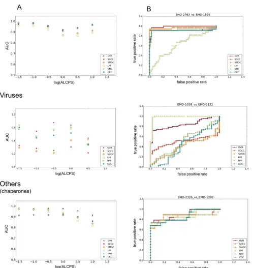
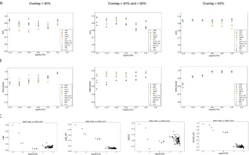
Using the distribution of fits from GMfit and the resultant ROC curves, we evaluated the ability of different scores to discriminate between true and false positives. We computed Area Under the Curve (AUC) of each score at different levels of required similarity to the reference alignment, as set by the ALCPS threshold (Fig. 2A). As the fit moves farther from the reference, the log10(ALCPS) values go from negative to positive. Similar orientations were usually observed for poses with log10(ALCPS) up to around 0.0 ± 0.5 (Fig. S2), i.e. small rotations and translations from the reference. For example, log10(ALCPS)0.0 roughly corresponds to a shift of 6 Å with a rotation of 10°, or a shift of 10 Å with a rotation of 6°. There is some variation in the performance of the scores with the choice of ALCPS threshold, depending also on the structural cate-gory. Hence we considered log10(ALCPS) thresholds specific for each category such that the threshold distinguishes the cluster of correct orientations for most of the fits in that category. We used threshold values of 0.82, 0.50 and0.40 for ribosomes, viruses and the category ‘others’, involving chaperones, respectively. The AUC shows different trends in each category, as the threshold is loosened (Fig. 2A). For ribosomes and viral maps, as the fits with correct orientation moved away from the reference fit, the AUC dropped initially before raising (Fig. 2A). This is largely due to the fact that at intermediate to low resolutions, an ensemble of similar orientations typically has comparable scores (Farabella et al., 2015; Goulet et al., 2014; Lukoyanova et al., 2015). On the other hand, the precision of scores generally improves for all struc-tural classes as the criterion for a good fit is weakened (Fig. S3). Nevertheless, in general our conclusions about the relative merits of different scores are independent of the ALCPS threshold used.
3.1. Differences in density distribution and composition
Dengue virus (EMD-5117) vs Dengue virus serotype 1 complexed with HMAb (EMD-5268)) (Figs. 2B and 3). For these and a few other viral map comparisons in the test dataset only a part of one map or parts of both maps were comparable reflecting partial overlap (Table 1). Hence a local score such as LMI is expected to be
better in such cases, due to the fact that the non-overlapping regions had significant differences.
[image:8.595.45.546.81.609.2]For the alignment between human enterovirus 71 (EMD-2436) (Plevka et al., 2014) and human poliovirus 3 (EMD-1562) (Zhang et al., 2008), two maps for which the density distributions are
not comparable, the AUC of SCCC was significantly higher than that of SMOC (Figs. 2B and3). Poliovirus is structurally similar to other enteroviruses, with a non-enveloped icosahedral protein coat encapsulating an RNA genome. The enteroviral volume core is empty compared to the high-density core of the polioviral map (Fig. 3A.ii & iii) and the capsids have similar diameters. The surface protrusions involving relatively lower density values are important in differentiating the correct alignment from the rest. Mean differ-ence in the region of overlap helped to match these low-density surface features (both negative after mean difference) with a raise in score (Fig. 3B.ii & iii). Equivalent minimal densities however have a relatively lower contribution to SMOC, which involves pro-duct of absolute densities.
3.2. Differences in surfaces
The two new filters applied for surface envelope detection (sur-face definition M and A, seeMethods) significantly improved AUC of surface-based scores, compared to those used previously which were based on a contour threshold range (surface definition T) (Farabella et al., 2015; Vasishtan and Topf, 2011) (Table 2). The selection of surface points in a range of contour thresholds (defini-tion T) is affected by the relative spatial varia(defini-tion of density levels at the surface. Considering all points on the iso-contour surface touching at least one exterior voxel (surface definition A) generally resulted in a better performance than the other surface envelope definitions (Fig. 4,Table 2).
The normalization of CD scores based on GDT-like weights improved their AUC values and precision, especially in the case of ribosomal and ‘others’ (Table 2,Figs. 4&S3). The normalized CDAgdt and CDMgdt scores had the best AUC and accuracies for
ribosomes, when compared to all the other scores (Table 2). Ribo-somes have unique and discernible surface features when com-pared to viral maps and those belonging to the category ‘others’.
Fig. S4B gives examples of cases from each category where the AUC of CD scores were comparable or better than other scores with good performance in each category. For example, in the case of viral map fit EMD-1058 (18 Å map of echovirus type 12 bound to a protein decay-accelerating factor (CD 55)) vs EMD-5122 (10 Å map of human poliovirus 1 RNA-releasing intermediate), the per-formance of CDMgdt score better than other scores except LMI, which also had a similar ROC curve. Though the echovirus is pack-aged, the maps have similar exposed surface features represented by viral proteins VP1 and VP3 (Fig. 1B andS4B). The CDMgdt score was effective in distinguishing alignments base on these exposed surface features (Fig. 1B).
In the selected dataset, there are many cases in the viral and chaperone map pairs where both outer and inner surfaces have sig-nificant differences due to nucleic acid packaging (e.g. EMD-2436 vs EMD-1562, EMD-5466 vs EMD-2397, EMD-1058 vs EMD-5122 etc), substrate binding (e.g. EMD-2325 vs EMD-2326) and confor-mational changes (e.g. EMD-5140 vs EMD-5248). NVA, which is calculated by comparing gradient normals at all surface points, has generally higher AUC and precision for viral maps (Table 2,
Fig. 4&S3), comparable to the best density-based scores. As the score works based on density gradient vectors, it is less affected by the differences in the location of selected surface voxels in com-parison to the CD scores.Fig. S5gives a few examples where the maps being compared have significant conformational differences. Even in these difficult cases of alignment, the surface based score NVA, is useful in discriminating the correct alignments from the rest.
3.3. Local vs global density-based scores
Local cross correlation (SCCC) was introduced to avoid the influ-ence of non-overlapping density in the calculations and quite a few developments that followed used this score (Roseman, 2000; Trabuco et al., 2008; Velazquez-Muriel et al., 2005). This is espe-cially relevant in the case of subunit matching where the density of other components contribute to global score calculations. Local score calculations do not suffer from these limitations but they do not account for the extent of overlap. In other words, a small overlapping segment can have a better correlation score than a rel-atively larger overlap. An example is shown inFig. S2, for the align-ment of viral maps: Enterovirus 71 empty capsid (EMD-5466) and Enterovirus 71 in complex with a neutralizing antibody E18 (EMD-2397). Some of the incorrect fits with minimal overlap get higher SCCC scores compared to correct orientations (log10(ALCPS) <1.0) with higher overlap. In terms of precision, SCCC was best for ribosomes and was among the top few scores for the group, ‘others’. (Table 2,Fig. S3).
3.4. Addition of overlap information to local scores
Generally, the fraction of overlap (OVR) score was good at dis-criminating between good and bad alignments across all structural categories, as judged by the AUC (Fig. 2), but had relatively lower precision (higher false positives) for the category ‘others’ including chaperones (Table 2). OVR score by itself is a good measure to dis-criminate correct alignments but is independent of voxel density values. Especially in case of subunit alignments or in the absence of significant surface features, one encounters solutions where most or all have large overlap with the target volume and hence OVR is less discriminatory in this context. An example from our dataset is the alignment of two ribosomal reconstructions: the par-tial yeast 48S preinitiation complex (EMD-2763) and E-coli 30S subunit in complex with the YjeQ biogenesis factor (EMD-1895). The reference alignment scored lower than the bad fits by OVR metric (Fig. S2). SCCC, however, picks the reference fit with the best score. Also, in theory, two different but similarly-sized sub-volumes will fit with the same overlap score at a specific region
of the target map. Hence a combination of correlation score with the overlap information could be more suitable. We calculated combined scores after scaling OVR relative to other scores (e.g. SCCC) by applying scale and shift factors as:
Scale factor¼median absolute de
v
iation of SCCC median absolute dev
iation of OVRShift factor¼ ðmedian of SCCCÞ ðmedian of OVRÞ
The OVR score was first scaled and then shifted by a shift factor.
OVR norm¼ ðOVRscale factorÞ þshift factor
The combined score is the average of scaled and shifted OVR (OVRnorm) and SCCC/SMOC/LMI.
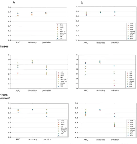
Inclusion of OVR information to the local scores (SCCC + OV, SMOC + OV and LMI + OV) improved the AUC significantly for all the three categories (Table 2,Fig. 4). These scores had comparable or better AUC and precision values than the best scores in each cat-egory (Table 2). LMI + OV (LMI_OV in theFig. 4) had better preci-sion than the other two correlation-based scores, especially in the case of viral maps.Fig. S4gives examples of cases from each category with the performance of different scores highlighted by ROC curves.
The combined scores were better than most other scores when the maps overlap partially (Fig. 5). Overall, the LMI + OV score had the best AUC for cases where only part of the maps match (<60% overlap) (Fig. 5A). In terms of precision, LMI + OV was also among the best scores (Fig. 5B). As mentioned above, global scores are as effective when major portions of the maps overlap (Fig. 5A&B).
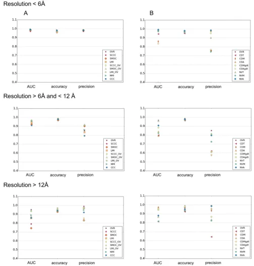
3.5. Performance at different resolution ranges
Analysis of different scores for their performance with maps at different resolution ranges (Fig. 6), shows that at resolutions better than 6 Å, all the density-based scores and OVR has similar AUC and precision (Fig. 6). At intermediate and low resolutions, the scores involving combination of SCCC, SMOC or LMI and OVR scores, had better AUC and precision than other scores. LMI + OV score (LMI_OV in the figure) was slightly better at low resolutions
com-Table 2
For the three map categories, the average AUC value, accuracy and precision of each score, are given. These were calculated at log10(ALCPS) thresholds selected for each category (ribosomes: 0.82, viruses:0.5, others:0.4). The scores which are better discriminatory and/or have higher precision, are in bold. OVR: Overlap score, LMI: Local mutual information, NMI: Normalized mutual information, SCCC: Local cross correlation, SMOC: Local cross correlation about zero. The combined scores with OVR are indicated with the ‘ +OV’ tag. CDT: Surface distance score on points selected based on a density threshold range. CDM: Surface distance score on points selected using mean filter (to identify more exposed regions), CDA: Surface distance score on all points at an iso-contour level, CDTgdt, CDMgdt & CDAgdt scores are normalized variants of CDT, CDM & CDA (see Methods), NVT: Normal vector score on surface points selected from a density threshold range, NVM: Normal vector score on surface points identified by mean filter on binary mask, NVA: Normal vector score on all points at an iso-contour level.
Scores Ribosome Virus Others
AUC Accuracy Precision AUC Accuracy Precision AUC Accuracy Precision
OVR 0.974 0.990 0.991 0.939 0.971 0.872 0.978 0.977 0.895
SMOC 0.931 0.957 0.979 0.707 0.933 0.705 0.964 0.969 0.970
SCCC 0.983 0.980 0.997 0.727 0.936 0.705 0.946 0.969 0.969
CCC 0.973 0.990 0.991 0.843 0.945 0.802 0.917 0.969 0.834
LMI 0.901 0.923 0.941 0.887 0.979 0.848 0.948 0.970 0.894
NMI 0.969 0.989 0.991 0.881 0.946 0.830 0.972 0.976 0.909
CDT 0.931 0.976 0.914 0.685 0.929 0.458 0.875 0.952 0.629
CDM 0.954 0.991 0.920 0.801 0.970 0.436 0.856 0.962 0.649
CDA 0.967 0.990 0.991 0.821 0.976 0.717 0.854 0.970 0.700
NVT 0.960 0.979 0.990 0.861 0.948 0.719 0.974 0.973 0.827
NVM 0.978 0.984 0.984 0.701 0.939 0.643 0.882 0.962 0.667
NVA 0.914 0.983 0.990 0.922 0.959 0.870 0.911 0.970 0.837
CDTgdt 0.921 0.971 0.833 0.741 0.935 0.461 0.875 0.952 0.629
CDMgdt 0.983 0.994 0.992 0.643 0.968 0.372 0.881 0.968 0.657
CDAgdt 0.969 0.990 0.991 0.860 0.976 0.748 0.935 0.971 0.690
SMOC + OV 0.976 0.989 0.991 0.852 0.942 0.710 0.976 0.976 0.976
SCCC + OV 0.982 0.990 0.991 0.854 0.961 0.736 0.974 0.975 0.970
pared to the combined scores involving SCCC or SMOC. This is lar-gely due to the fact that the MI scores use a coarser or binned rep-resentation of density, which is useful at these resolutions. Among the surface-based scores, NVA was better overall at both high (bet-ter than 6 Å) and in(bet-termediate resolutions (6–12 Å). CDAgdt score was better discriminatory at resolutions worse than 12 Å, apart from the combined scores.
3.6. Performance when fitting atomic components to maps representing a larger complex
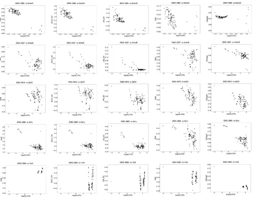
[image:11.595.68.549.83.587.2]We also tested the performance of different scores for discriminating the reference and near-optimal fits from incorrect fits when fitting a component of the complex represented by the map. We selected 5 cases spanning different resolutions
(Table S1). The fitted model associated with the map (in PDB) was considered as the reference fit and the component was fitted in the map using GMfit. While assessing the solutions from GMfit, we observed trends similar to that of the whole-map alignments where the density based scores were better at higher resolutions and the surface-based scores were more discriminatory at low res-olutions (Fig. 7). Only in the case EMD-5940 vs PDB 1rs9, where the crystal structure of nitric oxide synthase heme domains (dimer) were fitted into the low resolution (23 Å) map of calmodulin bound dimeric nitric oxide synthase, the density based scores failed and only the surface scores identified the correct fit (Yokom et al., 2014) (Fig. 7). The density-based and combined scores were less discriminatory at this resolution. LMI + OV was better across reso-lutions when compared to SCCC + OV (e.g. EMD-5610 vs 4chwB in
Fig. 7). As mentioned above, a simple OVR score is not effective as a general metric for cases of partial fits (e.g. EMD-5940 vs 1rs9, EMD-5610 vs 3j3rD).
3.7. Computational speed
All the scoring functions tested in this study (new scores and the improvements from our previous studies (Farabella et al., 2015; Vasishtan and Topf, 2011)) can be used to rank a set of align-ments generated by any density fitting method, and are suitable for comparing either two volumes or an atomic model and a volume at any resolution. They are all implemented in TEMPy (http://tempy. ismb.lon.ac.uk/). When applied to maps of size 300300300
using a single processor, the calculation takes: 0.5 s for LMI + OV (combined score) and CD (surface-based), 0.9 s for NVA (surface-based), and 0.05 for SCCC + OV (local density-based). The longer run-time of LMI + OV score can be attributed partly to the time for generation of binned density maps and calculation of frequencies, and also to the current Pythonic implementation. We plan to re-implement this metric in C, which will improve the speed of calculations.
4. Summary and recommendations
As part of a volume-matching pipeline that we have been devel-oping for 3D-EM data, we have tested various approaches to score alignments obtained from volume matching programs. We demon-strate that the performance of the different scoring functions varies depending on the shape and density composition of the assemblies represented by the map, the resolution and the extent of similarity or overlap.
[image:12.595.46.539.65.371.2]Overall, our results (summarised inFig. 8) show that combined scores are more effective as a general measure than the standard CCC, which is not the best discriminator across all resolutions or for partial overlaps. A combined score involving local mutual infor-mation and fraction of overlap (LMI_OV in the figure) is the best performing score in terms of AUC and precision across resolutions, map types and extents of overlap.We therefore recommend LMI_OV as the preferred scoring function for general use, while other scores may be useful for studies focused on particular cases.
Generally,density-based scoring functionsare influenced by the size and shape of the density distributions being compared while surface-based scoring functions are affected mainly by the extent of surface features and selection of contour. When comparing maps that typically have partial overlaps and significant composi-tional differences (e.g. viral maps), mutual information-based scores (NMI/LMI) are more discriminatory than
cross-correlation-based scores (CCC/SCCC/SMOC). However, for ribosomal maps and ‘others’, the local SCCC score has better precision, at high-to-intermediate resolutions in cases where the maps overlap to a large extent.
Surface-based scoring functions can also be useful at
[image:13.595.47.552.67.596.2]intermediate-to-low resolutions. We find that surface detection by selection of all points on the iso-contour (surface definition A)
Fig. 7.Scores vs ALCPS (log10scale), for cases of subunit model fits in maps. In the plots, each point represents one of the 100 fits generated by GMfit, except for the dot in the top left-hand corner which indicates the reference fit (The reference alignment is assigned a minimum log10(ALCPS) value of2.0 for the purpose of plotting). ALCPS measures the distance of a fit from the reference alignment, with lower values indicating better fits. See the Methods for an explanation of the different scores shown here.
[image:14.595.51.536.530.689.2]is generally more effective for such scores. Among these, the nor-mal vector score (NVA) calculated based on surface density gradi-ents, is more precise at different resolution ranges (mainly high-to-intermediate) especially when there are significant compositional and conformational differences (e.g. in the case of viruses and chaperones). The Chamfer distance (CDAgdt), which is based on distance between surface points, is better at low resolutions, where density variation is less informative. In the future, we plan to develop approaches to detect local surface matches (partial over-laps) and test the performance of the surface-based scoring func-tions on local surface regions.
In summary, we have analysed a wide variety of scoring func-tions for comparing EM maps taken from a range of structural classes with different shape, size and resolution. We also provided combined metrics that include the information on the extent of overlap between volumes. Based on our results, we recommend the combined score LMI_OV as having the widest applicability. This score is likely to be useful for comparing large datasets of density maps and models and for integrative structure modelling based on data at different resolutions.
Acknowledgements
We thank Dr. David Houldershaw for computer support, Joshua Bullock, and Drs. Tom Burnley and Irene Farabella for helpful dis-cussions. This work was undertaken as part of the BioMedBridges project, funded by the European Union Seventh Framework Pro-gramme within Research Infrastructures of the FP7 Capacities Specific Programme, grant agreement number 284209. We also thank MRC research grants MR/M019292/1 and MR/N009614/1.
Appendix A. Supplementary data
Supplementary data associated with this article can be found, in the online version, athttp://dx.doi.org/10.1016/j.jsb.2017.05.007.
References
Bai, X.C., Fernandez, I.S., McMullan, G., Scheres, S.H., 2013. Ribosome structures to near-atomic resolution from thirty thousand cryo-EM particles. eLife 2, e00461.
http://dx.doi.org/10.7554/eLife. 00461.
Birmanns, S., Wriggers, W., 2007. Multi-resolution anchor-point registration of biomolecular assemblies and their components. J. Struct. Biol. 157, 271–280.
http://dx.doi.org/10.1016/j.jsb.2006.08.008.
Ceulemans, H., Russell, R.B., 2004. Fast fitting of atomic structures to low-resolution electron density maps by surface overlap maximization. J. Mol. Biol. 338, 783– 793.http://dx.doi.org/10.1016/j.jmb.2004.02.066.
Chacon, P., Wriggers, W., 2002. Multi-resolution contour-based fitting of macromolecular structures. J. Mol. Biol. 317, 375–384. http://dx.doi.org/ 10.1006/jmbi.2002.5438.
Chen, Z., Husz, Z.L., Wallace, I., Wallace, A.M., 2007. Video Object Tracking Based on a Chamfer Distance Transform. IEEE International Conference on Image Processing, III-357-III-360. doi:10.1109/ICIP.2007.4379320.
Davis, J., Goadrich, M., 2006. The Relationship Between Precision-Recall and ROC Curves. ACM Press.http://dx.doi.org/10.1145/1143844.1143874, pp. 233-240. De-Alarcón, P.A., Pascual-Montano, A., Gupta, A., Carazo, J.M., 2002. Modeling shape
and topology of low-resolution density maps of biological macromolecules. Biophys. J. 83, 619–632.http://dx.doi.org/10.1016/S0006-3495(02)75196-5. Dugan, J.M., Altman, R.B., 2004. Using surface envelopes for discrimination of
molecular models. Protein Sci. 13, 15–24. http://dx.doi.org/10.1110/ ps.03385504.
Esquivel-Rodriguez, J., Kihara, D., 2012. Fitting multimeric protein complexes into electron microscopy maps using 3D Zernike descriptors. J. Phys. Chem. B 116, 6854–6861.http://dx.doi.org/10.1021/jp212612t.
Farabella, I., Vasishtan, D., Joseph, A.P., Pandurangan, A.P., Sahota, H., Topf, M., 2015. A Python library for assessment of three-dimensional electron microscopy density fits. J. Appl. Crystallogr. 48, 1314–1323. http://dx.doi.org/10.1107/ S1600576715010092.
Field, L., Suhr, S., Ison, J., Wouter, L., Wittenburg, P., Broeder, D., Hardisty, A., Repo, S., Jenkinson, A., 2013. Realising the full potential of research data: common challenges in data management, sharing and integration across scientific disciplines. Joint working paper by the FP7 ESFRI cluster projects: BioMedBridges, CRISP, DASISH, ENVRI. doi:doi:10.5281/zenodo.7636.
Garzon, J.I., Kovacs, J., Abagyan, R., Chacon, P., 2007. ADP_EM: fast exhaustive multi-resolution docking for high-throughput coverage. Bioinformatics 23, 427–433.
http://dx.doi.org/10.1093/bioinformatics/btl625.
Goddard, T.D., Huang, C.C., Ferrin, T.E., 2007. Visualizing density maps with UCSF Chimera. J. Struct. Biol. 157, 281–287. http://dx.doi.org/10.1016/j. jsb.2006.06.010.
Goulet, A., Major, J., Jun, Y., Gross, S.P., Rosenfeld, S.S., Moores, C.A., 2014. Comprehensive structural model of the mechanochemical cycle of a mitotic motor highlights molecular adaptations in the kinesin family. Proc. Nat. Acad. Sci. U.S.A. 111, 1837–1842.http://dx.doi.org/10.1073/pnas.1319848111.
Harpaz, Y., Gerstein, M., Chothia, C., 1994. Volume changes on protein folding. Structure 2, 641–649.
Henderson, R., Sali, A., Baker, M.L., Carragher, B., Devkota, B., Downing, K.H., Egelman, E.H., Feng, Z., Frank, J., Grigorieff, N., Jiang, W., Ludtke, S.J., Medalia, O., Penczek, P.A., Rosenthal, P.B., Rossmann, M.G., Schmid, M.F., Schroder, G.F., Steven, A.C., Stokes, D.L., Westbrook, J.D., Wriggers, W., Yang, H., Young, J., Berman, H.M., Chiu, W., Kleywegt, G.J., Lawson, C.L., 2012. Outcome of the first electron microscopy validation task force meeting. Structure 20, 205–214.
http://dx.doi.org/10.1016/j.str.2011.12.014.
Joseph, A.P., Malhotra, S., Burnley, T., Wood, C., Clare, D.K., Winn, M., Topf, M., 2016. Refinement of atomic models in high resolution EM reconstructions using Flex-EM and local assessment. Methods 100, 42–49.http://dx.doi.org/10.1016/j. ymeth.2016.03.007.
Kawabata, T., 2008. Multiple subunit fitting into a low-resolution density map of a macromolecular complex using a gaussian mixture model. Biophys. J. 95, 4643– 4658.http://dx.doi.org/10.1529/biophysj.108.137125.
Kuhlbrandt, W., 2014. Biochemistry. The resolution revolution. Science 343, 1443– 1444.http://dx.doi.org/10.1126/science.1251652.
Lagerstedt, I., Moore, W.J., Patwardhan, A., Sanz-Garcia, E., Best, C., Swedlow, J.R., Kleywegt, G.J., 2013. Web-based visualisation and analysis of 3D electron-microscopy data from EMDB and PDB. J. Struct. Biol. 184, 173–181.http://dx. doi.org/10.1016/j.jsb.2013.09.021.
Lukoyanova, N., Kondos, S.C., Farabella, I., Law, R.H., Reboul, C.F., Caradoc-Davies, T. T., Spicer, B.A., Kleifeld, O., Traore, D.A., Ekkel, S.M., Voskoboinik, I., Trapani, J.A., Hatfaludi, T., Oliver, K., Hotze, E.M., Tweten, R.K., Whisstock, J.C., Topf, M., Saibil, H.R., Dunstone, M.A., 2015. Conformational changes during pore formation by the perforin-related protein pleurotolysin. PLoS Biol. 13, e1002049.http://dx. doi.org/10.1371/journal.pbio.1002049.
Milne, J.L., Borgnia, M.J., Bartesaghi, A., Tran, E.E., Earl, L.A., Schauder, D.M., Lengyel, J., Pierson, J., Patwardhan, A., Subramaniam, S., 2013. Cryo-electron microscopy–a primer for the non-microscopist. FEBS J. 280, 28–45.http://dx. doi.org/10.1111/febs.12078.
Mukherjee, S., Zhang, Y., 2009. MM-align: a quick algorithm for aligning multiple-chain protein complex structures using iterative dynamic programming. Nucleic Acids Res. 37, e83.http://dx.doi.org/10.1093/nar/gkp318.
Pandurangan, A.P., Shakeel, S., Butcher, S.J., Topf, M., 2014. Combined approaches to flexible fitting and assessment in virus capsids undergoing conformational change. J. Struct. Biol. 185, 427–439.http://dx.doi.org/10.1016/j.jsb.2013.12.003. Pettersen, E.F., Goddard, T.D., Huang, C.C., Couch, G.S., Greenblatt, D.M., Meng, E.C., Ferrin, T.E., 2004. UCSF Chimera–a visualization system for exploratory research and analysis. J. Comput. Chem. 25, 1605–1612. http://dx.doi.org/10.1002/ jcc.20084.
Pintilie, G.D., Zhang, J., Goddard, T.D., Chiu, W., Gossard, D.C., 2010. Quantitative analysis of cryo-EM density map segmentation by watershed and scale-space filtering, and fitting of structures by alignment to regions. J. Struct. Biol. 170, 427–438.http://dx.doi.org/10.1016/j.jsb.2010.03.007.
Plevka, P., Lim, P.Y., Perera, R., Cardosa, J., Suksatu, A., Kuhn, R.J., Rossmann, M.G., 2014. Neutralizing antibodies can initiate genome release from human enterovirus 71. Proc. Nat. Acad. Sci. U.S.A. 111, 2134–2139.http://dx.doi.org/ 10.1073/pnas.1320624111.
Read, R.J., Chavali, G., 2007. Assessment of CASP7 predictions in the high accuracy template-based modeling category. Proteins 69 (Suppl 8), 27–37.http://dx.doi. org/10.1002/prot.21662.
Roseman, A.M., 2000. Docking structures of domains into maps from cryo-electron microscopy using local correlation. Acta crystallogr. Sect D: Biol. Crystallogr. 56, 1332–1340.
Rossmann, M.G., 2000. Fitting atomic models into electron-microscopy maps. Acta crystallogr. Sect D: Biol. Crystallogr. 56, 1341–1349.
Saha, M., Morais, M.C., 2012. FOLD-EM: automated fold recognition in medium- and low-resolution (4–15 A) electron density maps. Bioinformatics 28, 3265–3273.
http://dx.doi.org/10.1093/bioinformatics/bts616.
Saha, M., Levitt, M., Chiu, W., 2010. MOTIF-EM: an automated computational tool for identifying conserved regions in CryoEM structures. Bioinformatics 26, i301–i309.http://dx.doi.org/10.1093/bioinformatics/btq195.
Schneidman-Duhovny, D., Rossi, A., Avila-Sakar, A., Kim, S.J., Velazquez-Muriel, J., Strop, P., Liang, H., Krukenberg, K.A., Liao, M., Kim, H.M., Sobhanifar, S., Dotsch, V., Rajpal, A., Pons, J., Agard, D.A., Cheng, Y., Sali, A., 2012. A method for integrative structure determination of protein-protein complexes. Bioinformatics 28, 3282–3289. http://dx.doi.org/10.1093/bioinformatics/ bts628.
Shatsky, M., Hall, R.J., Brenner, S.E., Glaeser, R.M., 2009. A method for the alignment of heterogeneous macromolecules from electron microscopy. J. Struct. Biol. 166, 67–78.http://dx.doi.org/10.1016/j.jsb.2008.12.008.
Sturges, H.A., 1926. The choice of a class interval. J. Am. Stat. Assoc. 21, 65–66.
http://dx.doi.org/10.1080/01621459.1926.10502161.
Topf, M., Sali, A., 2005. Combining electron microscopy and comparative protein structure modeling. Curr. Opin. Struct. Biol. 15, 578–585. http://dx.doi.org/ 10.1016/j.sbi.2005.08.001.
Topf, M., Lasker, K., Webb, B., Wolfson, H., Chiu, W., Sali, A., 2008. Protein structure fitting and refinement guided by cryo-EM density. Structure 16, 295–307.
http://dx.doi.org/10.1016/j.str.2007.11.016.
Trabuco, L.G., Villa, E., Mitra, K., Frank, J., Schulten, K., 2008. Flexible fitting of atomic structures into electron microscopy maps using molecular dynamics. Structure 16, 673–683.http://dx.doi.org/10.1016/j.str.2008.03.005.
van Zundert, G.C., Trellet, M., Schaarschmidt, J., Kurkcuoglu, Z., David, M., Verlato, M., Rosato, A., Bonvin, A.M., 2017. The DisVis and PowerFit web servers: explorative and integrative modeling of biomolecular complexes. J. Mol. Biol. 429, 399–407.http://dx.doi.org/10.1016/j.jmb.2016.11.032.
Vasishtan, D., Topf, M., 2011. Scoring functions for cryoEM density fitting. J. Struct. Biol. 174, 333–343.http://dx.doi.org/10.1016/j.jsb.2011.01.012.
Velazquez-Muriel, J.A., Sorzano, C.O., Scheres, S.H., Carazo, J.M., 2005. SPI-EM: towards a tool for predicting CATH superfamilies in 3D-EM maps. J. Mol. Biol. 345, 759–771.http://dx.doi.org/10.1016/j.jmb.2004.11.005.
Villa, E., Lasker, K., 2014. Finding the right fit: chiseling structures out of cryo-electron microscopy maps. Curr. Opin. Struct. Biol. 25, 118–125.http://dx.doi. org/10.1016/j.sbi.2014.04.001.
Volkmann, N., Hanein, D., 1999. Quantitative fitting of atomic models into observed densities derived by electron microscopy. J. Struct. Biol. 125, 176–184.http:// dx.doi.org/10.1006/jsbi.1998.4074.
Wang, Z., Schroder, G.F., 2012. Real-space refinement with DireX: from global fitting to side-chain improvements. Biopolymers 97, 687–697. http://dx.doi.org/ 10.1002/bip.22046.
Woetzel, N., Lindert, S., Stewart, P.L., Meiler, J., 2011. BCL::EM-Fit: rigid body fitting of atomic structures into density maps using geometric hashing and real space
refinement. J. Struct. Biol. 175, 264–276. http://dx.doi.org/10.1016/j. jsb.2011.04.016.
Wriggers, W., 2012. Conventions and workflows for using Situs. Acta Crystallogr. Sect D: Biol. Crystallogr. 68, 344–351. http://dx.doi.org/10.1107/ S0907444911049791.
Xu, J., Zhang, Y., 2010. How significant is a protein structure similarity with TM-score = 0.5? Bioinformatics 26, 889–895. http://dx.doi.org/10.1093/ bioinformatics/btq066.
Yokom, A.L., Morishima, Y., Lau, M., Su, M., Glukhova, A., Osawa, Y., Southworth, D. R., 2014. Architecture of the nitric-oxide synthase holoenzyme reveals large conformational changes and a calmodulin-driven release of the FMN domain. J. Biol. Chem. 289, 16855–16865.http://dx.doi.org/10.1074/jbc.M114.564005.
Zemla, A., 2003. LGA: a method for finding 3D similarities in protein structures. Nucleic Acids Res. 31, 3370–3374.
Zemla, A., Geisbrecht, B., Smith, J., Lam, M., Kirkpatrick, B., Wagner, M., Slezak, T., Zhou, C.E., 2007. STRALCP–structure alignment-based clustering of proteins. Nucleic Acids Res. 35, e150.http://dx.doi.org/10.1093/nar/gkm1049. Zhang, P., Mueller, S., Morais, M.C., Bator, C.M., Bowman, V.D., Hafenstein, S.,
Wimmer, E., Rossmann, M.G., 2008. Crystal structure of CD155 and electron microscopic studies of its complexes with polioviruses. Proc. Nat. Acad. Sci. U.S. A. 105, 18284–18289.http://dx.doi.org/10.1073/pnas.0807848105.
Zhang, S., Vasishtan, D., Xu, M., Topf, M., Alber, F., 2010. A fast mathematical programming procedure for simultaneous fitting of assembly components into cryoEM density maps. Bioinformatics 26, i261–i268.http://dx.doi.org/10.1093/ bioinformatics/btq201.
Zhang, Y., Skolnick, J., 2004. Scoring function for automated assessment of protein structure template quality. Proteins 57, 702–710. http://dx.doi.org/10.1002/ prot.20264.