Volume: 03 Issue: 07 | July-2016 www.irjet.net p-ISSN: 2395-0072
© 2016, IRJET | Impact Factor value: 4.45 | ISO 9001:2008 Certified Journal | Page 1391
Efficient Maximum Power Point Tracking for a Distributed PV System under
Rapidly Changing Environmental Conditions
MOPURU BHARGAVI PG Student –ABIT, Siddavatam, Kadapa, Andra Pradesh, India BOGGAVARAPU RAMESH KUMAR H.O.D- ABIT, Siddavatam, Kadapa, Andra Pradesh, India Abstract
When conventional maximum power point
tracking(MPPT) techniques are required to operate fast under rapidly changing environmental conditions, a large power loss can becaused by slow tracking speed, output power fluctuation, or additionally required ad hoc parameters .This paper proposes a fast and efficient MPPT technique that minimizes the power loss with the adaptively binary-weighted step (ABWS) followed by the monotonically decreased step (MDS) without causing output power fluctuation nor requiring additional ad hoc parameter. The proposed MPPT system for a photovoltaic (PV) module is implemented by a boost converter with a microcontroller unit. The theoretical analysis and the simulation results show that the proposed MPPT provides fast and accurate
tracking under rapidly changing environmental conditions. The experimental results based on a distributed PV system demonstrate that the proposed MPPT technique is superior to the conventional perturb and observe (P&O) technique, which reduces the tracking time and the overall power loss by up to 82.95%,91.51% and 82.46%, 97.71% for two PV modules, respectively.
Index Terms—Binary-weighted step, distributed
system, environmental conditions, maximum power point (MPP), photovoltaic (PV) system.
1. INTRODUCTION:
As the costs of fossil fuels and their environmental concerns rise, the demand for innovation in renewable energy grows. In conventional photovoltaic (PV) systems using central or string inverters, each PV module array is connected to an inverter that uses passive components such as large capacitors and inductors. Mismatch and partial shading problems among PV modules connected in series are the primary sources of the power loss [1–3]. In order to mitigate these problems, a maximum power point tracking (MPPT) controller can be embedded into an inverter. To
further increase the energy that can be harvested, distributed PV systems with an MPPT for each PV module have been widely researched [4–11].An MPPT controller in a distributed PV system uses the
I–V characteristics of a PV module for tracking the
maximum power point (MPP) of its own module. Various MPPT techniques have been researched, and they can be categorized into three types: single step, multivariable step, and binary-weighted step. Previously described simple single-step techniques include perturp band observe (P&O) in [12], P&O
based on a PI controller in[13], [14], dP-P&O in [15],
incremental conductance (INC) in[16], power-increment-aided INC (PI-INC) with a two-phased tracking in [16], and the improved particle swarm optimization method in [17] and [18]. The main drawback of the single-step algorithms is their relatively slow tracking speed. Moreover, the operating point fluctuates around the MPP at the steady state, which may cause a large amount of available energy to be wasted. Even though P&O based on a PI controller minimizes the fluctuation by using a closed-loop control with a lower modulation frequency, the single-step algorithms are not
appropriate for rapidly changing environmental conditions. The multivariable-step algorithms adopt
a coarse-to-fine step at the expense of an ad hoc
Volume: 03 Issue: 07 | July-2016 www.irjet.net p-ISSN: 2395-0072
© 2016, IRJET | Impact Factor value: 4.45 | ISO 9001:2008 Certified Journal | Page 1392 the problem of output fluctuation is yet to be
resolved. Another MPPT technique for fast tracking based on the output power binary weighted step (BWS) is the successive approximation register (SAR)
MPPT in [25]. However, the periodic operation between its active and power-down modes inherently makes the output fluctuate even in the
absence of a change in environmental conditions. Moreover, the MSB operation runs first in the SAR MPPT, which increasingly aggravates the overall power loss. This paper presents an MPPT algorithm based on the adaptively binary-weighted step (ABWS) and the monotonically decreased step (MDS). The proposed MPPT technique detects the
MPP quickly without fluctuation or an additional ad
hoc parameter by using LSB first operation, which
allows for superior
performance compared to others in the tracking and the power loss not only under the steady state (normal operation)but also under the dynamic state (tracking operation). Besides, the lifetime of the components in the MPPT controller can be prolonged [26]. The proposed MPPT technique is implemented by employing a boost converter with a
microcontroller unit. The simulation and
experimental results are presented for validation.
I. CHARACTERISTICS OF A PV MODULE
As shown in Fig. 1(a), a PV cell can be represented by An equivalent circuit expressed as in [27]
Is = IPh − ID – Ish
= IPh − IS ·_eV + I ·R Sn ·V T − 1_− V + I · RS.RSh(1
Is = IPh − ID − ISh
= IPh − IS ·_eV + I ·N ·R Sn ·V T·N − 1− V + I · N · RSN RSh(2)
where I and V are redefined as the module current
and the voltage across the PV module, respectively. N is the number of cells in series. The power generated by a PV module depends on the current and voltage relationship. Especially under rapid environmental
changing conditions, IPh depends strongly on the
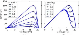
irradiance changes and partial shading conditions, which results in a change in power as shown in Fig. 2. Fig. 2(a) shows the decrease in the voltage at the MPP (VMPP) and the open-circuit voltage (VOC) of a PV module as the irradiance is reduced. The values of the irradiance are obtained from the method to extract the California Energy Commission (CEC) weighted
efficiency. In Fig. 2(b), VMPP is changed according to
the amount of shading in a PV cell at the irradiance of 1 Sun. The greater the number of shaded cells, the larger the variation in VMPP is. Most of conventional MPPT methods cause a fluctuation in the MPP after the tracking operation is completed, which increases power loss in the steady state. The I–V relationship at the MPP
Fig. 2. Power versus voltage characteristics of a PV module (a)under various irradiance conditions and (b) with a partially shaded cell.
can be defined as in [5]
I = ˆ V · ∂I∂V____MPP+ ˆ S · ∂I∂S____MPP+ ˆ T ·
∂I∂T____MPP(3)
where ˆx represents the small signal variation of x, S
the irradiance, and T is the temperature of a PV
module. Neglecting the variation of the irradiance and temperature in the steady state,(3) can be expressed as
PMPP = VMPP · IMPP − v2MPPRMPP(4)
where VMPP and IMPP include the fixed value at the
[image:2.612.326.496.377.452.2]Volume: 03 Issue: 07 | July-2016 www.irjet.net p-ISSN: 2395-0072
© 2016, IRJET | Impact Factor value: 4.45 | ISO 9001:2008 Certified Journal | Page 1393 and the voltage of the PV module, it is necessary for
an MPPT controller to promptly track the MPP and to maintain it with less fluctuation. There can be a tradeoff between the resolution of the tracking step and the tracking speed. In the next section, three MPPT techniques are analyzed and compared.
III. CONVENTIONAL MPPT TECHNIQUES
Perturb and Observe MPPT The procedure to track the MPP for the P&O algorithm is explained as follows. An MPPT controller first measures the input voltage and the current from a PV module. Then, the present power calculated by the controller is compared with previous power. Depending on the values of the present power and the previous power, the MPPT controller changes the input voltage of the PV module by controlling the duty of the pulse width modulation (PWM). In order to track the MPP, the controller needs to determine the increase or decrease of the duty that will result in a higher power. If the present power is larger than the previous power, the P&O algorithm maintains the same direction for controlling the duty, and vice versa. The P&O algorithm is simple to implement, but its slow tracking does not allow it to be applied under rapidly changing environmental conditions [28].
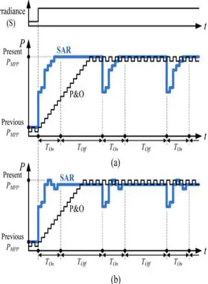
Fig 3. Comparison between P&O and SAR MPPT under the given irradiance conditions where the
power difference is for (a) 2N and (b) 2N – 2 with a 4-bit resolution.
The Successive Approximate Register (SAR) MPPT algorithm musing the BWS includes an active mode and a power down mode that alternate periodically [25]. In the active mode, the SAR
operation tracks the MPP with n-bit voltage
resolution. In each the iteration, a bit sequence of the voltage is determined from the MSB to the LSB. After determining each bit, one step is added for detecting the direction of voltage, i.e., whether the voltage should be increased or decreased. Because the SARMPPT algorithm uses the BWS—unlike the P&O algorithm, which tracks the MPP with a single step— the tracking speed is faster than that of the P&O algorithm. The computational cost for the P&O and
the SAR MPPT are 2n + 4 and2n − 1, respectively.
During the power-down mode, the SARMPPT retains the final voltage attained in the previous active mode. The SAR MPPT allows for fast tracking without fluctuation around the MPP. However, one of the main drawbacks of this method becomes apparent when keeping the voltage in the power-down mode. Even though the MPP is not changed, the periodic operation of the active and power-down modes changes the output voltage of the PV module as shown in Fig. 3(a) and(b). To reduce unnecessary power loss with the SAR MPPT, the power-down mode should be maintained for a longer duration than the active mode, but this will result in non detection of a new MPP that is changed rapidly in the power-down mode. Therefore, the operation of the SAR MPPT is not suitable for rapidly changing environment conditions. Moreover, the voltage fluctuation caused by periodic tracking of the MPP degrades the total harmonic distortion (THD) when connected to an inverter. Additionally, a minor drawback is that there is a probability of missing the MPP in the active mode by at least 1 LSB owing to the fixed number of tracking iterations, as depicted in Fig. 3(b).
[image:3.612.76.227.469.675.2]Volume: 03 Issue: 07 | July-2016 www.irjet.net p-ISSN: 2395-0072
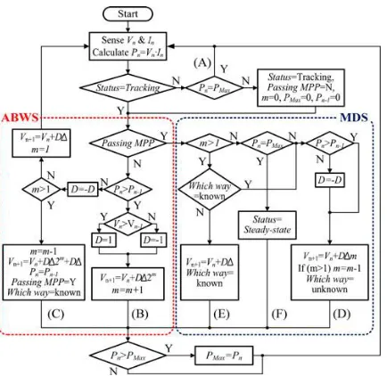
[image:4.612.39.256.104.315.2]© 2016, IRJET | Impact Factor value: 4.45 | ISO 9001:2008 Certified Journal | Page 1394 Fig 4. Flow chart of the proposed algorithm using
ABWS and MDS.
IV. IMPLEMENTATION OF THE PROPOSED ALGORITHM USINGABWS AND MDS
A. Description of the Proposed Algorithm
The MPP of a PV module varies according to the environmental conditions as discussed earlier. In order to reduce the power loss under rapidly changing environment conditions, the proposed algorithm aims at tracking the MPP as quickly as
possible. After tracking the MPP is completed, VMPP
remains unchanged as long as the environmental conditions are stable. The proposed MPPT algorithms are based on the ABWS and the MDS, which tracks the MPP quickly without the aforementioned problems caused by the P&O and the SAR MPPT. Similar to the BWS, the ABWS tracks the MPP by increasing the voltage tracking step in a binary manner but starts from the LSB with the minimum voltage tracking step Δ in Fig. 4. After a certain number of iterations, the operating voltage passes VMPP. Then, the ABWS stops and the MDS deploys to find the exact MPP. Unlike the fixed number of iterations in the SAR MPPT using the BWS, the number of iterations for tracking the MPP in the proposed MPPT algorithm is adaptively adjusted depending on the environmental condition change.
The ABWS passes an internal parameter to the MDS. From the next iteration right after the ABWS, the voltage step is then monotonically reduced until the
MPP is found. If the variation of the VMPP drops
below 1 LSB resolution, VMPP remains unchanged
and the MDS operation is terminated. The proposed MPPT algorithm enhances the tracking speed with less power loss for its fast tracking without output power fluctuation under the stable
Fig. 5. MPP tracking procedure in the normal case.
environmental condition. Additionally, the THD issue in SARMPPT can be resolved by using the proposed MPPT since the ABWS starts only when the environmental condition changes. The flowchart of the proposed algorithm is depicted in Fig. 4.At the nth iteration, the current “In ” and the voltage “Vn” of a PV module are sensed to calculate the output power “Pn” of the PV module. The variable “Status” is set to either “Tracking” or the “Steady-state” and indicates if
the proposed algorithm tracks or maintains VMPP.
The initial value for “Status” is setto “Tracking.” The variable “Passing MPP” is set to “Y” after a certain number of the ABWS iterations, which terminates the ABWS operation and activates the MDS operation sequentially after the MPP is passed. The variables “m” and “D” represent the exponent for the voltage
step increment and the direction of VMPP,
respectively. The variable “Which way” is used for
checking the correct direction of VMPP in each
Volume: 03 Issue: 07 | July-2016 www.irjet.net p-ISSN: 2395-0072
© 2016, IRJET | Impact Factor value: 4.45 | ISO 9001:2008 Certified Journal | Page 1395 available is unchanged as the current input power Pn
equals to the maximum power PMax. Thus, it still
falls into the steady-state operation. In this stage, the proposed algorithm simply continues to sense the input power as indicated in branch (A) in Fig. 4. In the iteration 1, the maximum power of a PV module moves to a higher voltage than the previous one. In
other words, Pn differs from PMax due to
environmental condition change. Then, the variable “Status” changes to “Tracking” as branch (B). The proposed algorithm starts tracking a new maximum
power PMPP by using the ABWS algorithm. If the
change of the operating voltage through branch (B) increases the power, the voltage step is continuously increased in the same direction “D” by the ABWS until it passes the MPP. Since the operating voltage at the iteration 4 causes reduction in the output power compared to the previous iteration, the direction of the change in the operating voltage is reversed and the operating voltage is decreased back to the
operating voltage of the previous iteration plus D·Δ
through branch (C) at iteration 5.
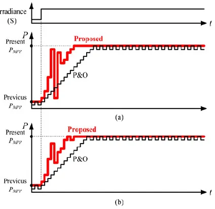
Fig. 6. Comparison between P&O and the proposed MPPT algorithm. The
conditions in (a) and (b) are the same as in Fig. 3(a) and (b).
Then, the MDS algorithm runs through branch (D) to reduce the operating voltage monotonically until it
becomes to the unit step Δ. The initial value of “m” in the MDS is obtained from the value of “m” set by the ABWS, and the operating voltage from the PV module
is changed by D·Δ·m at iteration 6. The proposed
algorithm operates until it finds the MPP with “Δ” when “m” is equal to 1. For each MDS operation, the correct direction “D” of the change in the operating voltage is checked through the branch (E) at iteration 7 and 9. At the iteration 11, the MPP can be detected if the present power PN equals to the temporary
maximum power PMax through branch (F). Finally,
the proposed algorithm stops by setting the variable “Status” to a
“Steady-state.” From the above discussion, the total
number of tracking iterations N Worst in the worst
case can be calculated from the following equation: N Worst = 2· n + 2n−1 − (n − 1) · n2+ 4 (5)
where n is the resolution. Fig. 6 illustrates the
comparison between the P&O and the proposed algorithm with 4-bit power resolution. The proposed algorithm tracks the MPP robustly without fluctuation, resulting in reduced power loss within 1-bitin the steady-state operation (2-bit power loss can be caused by the P&O algorithm). Therefore, the proposed MPPT algorithm tracks the MPP fast
without an ad hoc, which reduces the power loss of
PV modules without causing PV module dependency.
B. Proposed MPPT Algorithm With a Boost
Converter
Fig. 7 shows an example of the implementation for the proposed MPPT system dedicated to a distributed PV system. This system comprises a voltage divider, an inductor, capacitors, a diode, a power MOSFET, a current sensor, a buffer, and a micro controller unit (MCU). The boost converter controls the output voltage of a PV module by using the PWM from the MCU according to sensed values of the voltage and current of the PV
[image:5.612.40.252.402.608.2]Volume: 03 Issue: 07 | July-2016 www.irjet.net p-ISSN: 2395-0072
[image:6.612.36.257.105.205.2]© 2016, IRJET | Impact Factor value: 4.45 | ISO 9001:2008 Certified Journal | Page 1396 Fig. 7. Example of the implementation for the
proposed MPPT algorithm.
module. Since the voltage range of the PV module is from 6 to20 V, resistive dividers at the input and the output of the boost converter are necessary to divide the voltages by ten in order for the allowed voltage of the MCU input level. This study uses a PWM frequency of 125 kHz.
V. SIMULATION RESULTS
On the basis of the experimental results from a PV module(JSM100-36-01) that consists of 36 cells in series, the simulation results compare five MPPT algorithms: the P&O MPPT, the SAR MPPT, the MAHC MPPT, VSSINC MPPT, and the proposed MPPT. Fig. 8 shows the operating voltage and power of the PV module for various algorithms in the time domain while changing the irradiance from 1000 to 800 W/m2 at the62th iteration. The MPP tracking of the P&O, the MAHC, and the VSSINC MPPT takes more iterations for the initial setup compared with the tracking time of the proposed MPPT, resulting in more power loss due to low tracking speed and fluctuation around MPP. Even though the tracking time of the SAR MPPT is faster than that of the proposed MPPT, a large amount of power loss is introduced by the SAR MPPT due to the tracking allowed only in the active mode. Note that the active and power-down modes in the SAR MPPT are periodically repeated every 44 iterations in the simulation. For the situation where the change of the irradiance from 1000 to 800 W/m2, the tracking time of all algorithms are comparable with each other except for the SAR MPPT that takes longer. The difference in tracking time results in the difference in power loss. Fig. 9 shows the normalized power loss of five algorithms during dynamic tracking operation for the initial setup and the change of the irradiance
situation, where the power loss is normalized to the ideal power with the longest tracking timet1 of the
P&O and t2 of the SAR in Fig. 8, respectively. Here,
the normalized power loss PN loss for each MPPT
algorithm is defined as
PN loss =_ki=0 Pideal −_ki=0 P_ki=0 Pideal (6) where k is the number of the iterations.
Even if the SAR MPPT has very low normalized power loss among five algorithms under the initial setup, the periodically required active and power-down modes of the MPPT increases the overall power loss. Thus, by excluding the SAR, the normal-
[image:6.612.325.539.354.513.2]ized power loss of the proposed algorithm is superior to other algorithms under the initial setup. For normalized power loss under the variation of the irradiance from 1000 to 800 W/m2,the proposed algorithm is comparable to others within 0.03%variation.
Fig. 8. Simulated results for P&O, SAR, MAHC, VSSINC, and the proposed algorithms when the irradiance changes.
Volume: 03 Issue: 07 | July-2016 www.irjet.net p-ISSN: 2395-0072
[image:7.612.37.245.248.370.2]© 2016, IRJET | Impact Factor value: 4.45 | ISO 9001:2008 Certified Journal | Page 1397 Fig. 9. Normalized power loss for dynamic tracking
(a) initial setup duringt1 and (b) 20% irradiance drop during t2 .
[image:7.612.325.542.429.517.2]Based on the simulation results in Fig. 8, the overall l power loss for each algorithm with various voltage resolutions is shown in Fig. 10(a). The proposed MPPT algorithm reduces the overall power loss up to 81.96%, 26.95%, 35.6%, and 52.6%
Fig. 10. Simulated results for (a) overall power loss and (b) THD according
to the resolutions.
compared with the P&O, the SAR, the MAHC, and the VSSINCMPPT, respectively. The power loss of the proposed algorithms is obtained from 2.52% and 1.6% at 8-bit and 5-bit resolutions, respectively. The proposed algorithm is superior to other algorithms in terms of power loss at least 0.48% higher than others.
Fig. 10(b) shows the THD induced by the output power fluctuation of a PV module for each MPPT algorithm based on the simulation setup in Fig. 8.The periodic MSB switching operation of the SAR MPPT algorithm degrades the THD (>7%). However, the industrial standard for the THD in a grid-tied system is less than 5%[29], which indicates that the SAR MPPT algorithm cannot provide the stable power and be applied under rapidly changing environmental conditions. The THD, higher than 3%, can be occurred in the P&O, the MAHC, and the VSSINC MPPT below 5-bit resolution. In the proposed MPPT algorithm, however, no THD occurs regardless of the
resolution because the VMPP remains stable without
fluctuation under stable environmental condition. In order for the P&O, the SAR, the MAHC, and the VSSINC to maximize the power of a PV module, each MPPT should be adjusted for ad hoc parameters such as the minimum voltage step and the gain of variable step. Thus, PV module dependency cannot be avoided. On the other hand, the proposed MPPT can be applied to various types of PV modules without any ad hoc parameter as shown in Table I. As a result, simulation results validate that the proposed algorithm offers the lowest power loss and THD compared with the other algorithms regardless of resolution.
VI. EXPERIMENTAL RESULTS
[image:7.612.325.540.582.666.2]The proposed MPPT system is implemented with a boost converter as shown in Fig. 11. Two kinds of PV modules are mounted on a structure with a tilting angle of 40° for testing a distributed MPPT system. The azimuthal angle is manually adjusted to track the sun. Fig. 12 shows the experimental setup. Each PV module is connected to its own proposed MPPT system.
Fig. 11. MPPT system for implementing the proposed algorithm: (a) top and (b) bottom.
Volume: 03 Issue: 07 | July-2016 www.irjet.net p-ISSN: 2395-0072
© 2016, IRJET | Impact Factor value: 4.45 | ISO 9001:2008 Certified Journal | Page 1398 that transfers the data to the laptop and the
oscilloscope through serial port communication and SMA cables, respectively. At each iteration, the in-house real-time monitoring system stores the voltages and currents of a boost converter from the input and he output. The specifications of the two PV
modules (JSM100-36-01, SM-100PC8) are VMPP =
[image:8.612.35.260.506.607.2]17.64 V, VMPP = 19 V, and IMPP = 5.70 A, and IMPP = 5.27 A, respectively, under the standard testing condition (1000 W/m2 and 25 °C). The experiment evaluates the tracking time for the initial setup and the 20% irradiance drop. Because it is difficult to control their radiance rapidly for outdoor testing, the experiment controls the photocurrent by using partial shading technique instead [30].Experiments begin with fully shaded the PV modules. As shown in Fig. 13, three testing scenarios are sequentially performed for each PV module as follows:
Fig. 13. Procedure of the test scenarios I, II, and III.
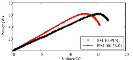
Fig. 14. P–V curves that are measured under 945 W/m2: the output power of each PV module (fully un shaded).
Scenario I: After being fully shaded, a PV module is fully un shaded.
Scenario II: Only one of the PV cells is partially shaded (20%)by placing a mask on top of the PV cell.
Scenario III: The mask is removed from the PV cell, which makes the fully un shaded condition for the PV module. Two algorithms, the P&O and the proposed, are tested on a sunny day and downloaded to the MCU one by one. The SARMPPT is not implemented because the period between the active mode and the
power-down mode is an ad hoc parameter that’
strongly affects the overall performance. The same experimental procedures are applied to all three scenarios as follows:
1) upload the P&O algorithm to the MPPT system; 2) acquire the current, voltage, and tracking time continuously under the testing condition;
3) upload the proposed algorithm to the MPPT system within10 s;
4) repeat step 2 for the proposed algorithm;
5) measure the tracking time and efficiency for each algorithm;
6) repeat steps from 1 to 5 for various resolutions .The ambient temperature at the time of testing is 22.8 °C,
[image:8.612.326.496.507.606.2]which leads to VMPP = 15.27 V, VMPP = 12.94 V and IMPP =4.02 A, IMPP = 4.77 A. In Fig. 14, P–V curves measured from two PV modules are shown under fully un shaded conditions at the irradiance of 945 W/m2. The efficiency of the boost converter is shown in Fig. 15 that exhibits the efficiency up to 98.89%. Figs. 16 and 17 depict the voltage across the PV modules (JSM100-36-01 and SM-100PC08) for three testing.
Volume: 03 Issue: 07 | July-2016 www.irjet.net p-ISSN: 2395-0072
[image:9.612.322.544.101.418.2]© 2016, IRJET | Impact Factor value: 4.45 | ISO 9001:2008 Certified Journal | Page 1399 Fig. 16. Voltage across a PV module for three
experimental sequences with7-bit resolution (JSM100-36-01):
(a) scenario I: initial setup, (b) scenario II: one cell partially shaded, and (c) scenario III: completely un shaded.
[image:9.612.326.544.506.686.2]scenarios. The tracking of MPPs for the P&O and the proposed are measured at the duty resolution of 7 bits, which allows for the 128 different values of duty ratio. The waveforms validates that the proposed algorithm can track the new MPP under partial shading conditions. It is clear that the proposed MPPT is faster than the P&O while maintaining the MPP without fluctuation. Based on the experimental results from Figs. 16 and 17, the analysis of the tracking time and dynamic tracking efficiency for the P&O and the proposed are presented for three testing scenarios with various duty resolution in Figs. 18 and 19.
Fig. 17. Voltage across a PV module for three experimental sequences with7-bit resolution (SM-100PC08): (a) scenario I: initial setup, (b) scenario II: one cell partially shaded, and (c) scenario III:
completely shaded.
Volume: 03 Issue: 07 | July-2016 www.irjet.net p-ISSN: 2395-0072
[image:10.612.325.543.298.454.2]© 2016, IRJET | Impact Factor value: 4.45 | ISO 9001:2008 Certified Journal | Page 1400 Fig. 18. Tracking time and dynamic tracking
efficiency for the three scenarios (JSM100-36-01): (a) and (c) P&O and (b) and (d) the proposed algorithm.
Regardless of PV module and scenario, the P&O exhibits a lower tracking efficiency and hence more power loss as the duty resolution increases due to the slow tracking time. The longest tracking time of the proposed MPPT is shorter than the shortest tracking time of the P&O, which makes the proposed
Fig. 19. Tracking time and Dynamic tracking
efficiency for the three scenarios (SM-100PC08): (a) and (c) P&O and (b) and (d) the proposed algorithm.
Fig. 20. Overall power loss for scenario I: (a) JSM100-36-01 and (b) SM-100PC08.
MPPT achieves a higher tracking efficiency compared to the P&O throughout various duty resolutions. The tracking time of the proposed MPPT is reduced by up to 82.95% and 82.46% for the PV modules JSM100-36-01 and SM-100PC08, respectively .Also, the dynamic tracking efficiency can be improved by up to 47.2% and 52.74%. Fig. 20 presents the overall power loss based on the experimental results from Figs. 16 and 17, which include both the dynamic tracking and the steady-state for two types of PV modules. The power loss of the P&O increases as the
duty resolution increases due to the decreased step size, whereas that of the proposed MPPT is comparable for all duty
resolutions presented. The proposed MPPT reduces the power loss up to 91.51% and 97.71% compared with the P&O MPPT. The experimental results confirm that the proposed MPPT algorithm is superior to the conventional P&O algorithm in regard to the tracking time and the overall power loss. Also, the PV module dependency is not presented in the proposed MPPT. Table II summarizes the MPPT performance of two different types of PV
[image:10.612.38.257.439.525.2]modules in a distributed PV system with two different MPPT
Fig 21 : Normalized power loss of dynamic tracking for three scenarios with7-bit resolution: (a) and (b) JSM100-36-01 and (c) and (d) SM-100PC08.
algorithms, while each MPPT algorithm is simultaneously performed for two PV modules. Due to the inherent fluctuation of the output power, the peak MPPT efficiency of the P&O algorithm is lower than that of the proposed algorithm even though the resolution is the same. The normalized power loss for three scenarios during tracking state is provided for the P&O and the proposed MPPT algorithms at 7-bit duty resolution as shown in fig.
CONCLUSION:
Volume: 03 Issue: 07 | July-2016 www.irjet.net p-ISSN: 2395-0072
© 2016, IRJET | Impact Factor value: 4.45 | ISO 9001:2008 Certified Journal | Page 1401 techniques, the ABWS and the MDS, minimize the
power loss under rapidly changing environmental
conditions without an additional ad hoc parameter.
Even though the proposed MPPT system is implemented by using a boos tconverter, it can also be applied to any type of DC-DC converter. The theoretical analysis and the simulation results validate that the proposed MPPT is superior to others. The experimental results quantify the performance enhancement of the proposed MPPT compared to the P&O in regard to the tracking time and the overall power loss not only under normal conditions but also
under rapidly changing environmental conditions.
REFERENCES:
[1] Y. S. Kim, S.-M. Kang, and R. Winston, “Modeling of a concentrating photovoltaic system for optimum land use,” Progress Photo voltaics: Res.
Appl., vol. 21, no. 2, pp. 240–249, Mar. 2013.
[2] Y. S. Kim, S.-M. Kang, and R. Winston, “Tracking control of high-concentration photovoltaic systems for minimizing power losses,”
Progress Photo voltaics: Res. Appl., vol. 22, no. 9, pp. 1001–1009, Sep.2014.
[3] Y.-H. Ji, D.-Y. Jung, J.-G. Kim, J.-H. Kim, T.-W. Lee, and C.-Y. Won, “A real maximum power point tracking method for mismatching compensation in
PV array under partially shaded conditions,” IEEE
Trans. Power Electron. vol. 26, no. 4, pp. 1001–1009,
Apr. 2011.
[4] R. C. N. Pilawa-Podgurski and D. J. Perreault, “Sub-module integrated distributed maximum power point tracking for solar photovoltaic applications,”
IEEE Trans. Power Electron., vol. 21, no. 8, pp. 2957– 2967,Jun. 2013.
[5] Y. S. Kim and R. Winston, “Power conversion in concentrating photovoltaic systems: Central, string, and micro-inverters,” Progress Photo voltaics:
Res. Appl., vol. 22, no. 9, pp. 984–992, Sep. 2014. [6] A. K. Abdel salam, A. M. Massoud, S. Ahmed, and P. N. Enjeti,
“High-performance adaptive perturb and observe
photovoltaic-based micro grids,” IEEE Trans. Power
Electron., vol. 26,
no. 4, pp. 1010–1021, Apr. 2011.
[7] D. Shmilovitz and Y. Levron, “Distributed maximum power point tracking in photovoltaic systems—Emerging architectures and control
methods,” Automatika—J. ControlMeas. Electron.
Comput. Commun., vol. 53,no. 2, pp. 142–155, 2012. [8] D.Meneses, O. Garcia, P. Alou, J. Oliver, R.Prieto, and J. Cobos, “Single stage grid-connected forward micro inverter with constant off-time boundary mode
control,” in Proc. IEEE Appl. Power Electron. Conf.
Expo., Feb. 2012, pp. 568–574.
[9] C. Deline, B. Marion, J. Granata, and S. Gonzales, “A performance and economic analysis of distributed power electronics in photovoltaic systems, ”Nat. Renew. Energy Lab., Golden, CO, USA, NREL Tech. Rep. NREL/TP-5200-50003, 2011.
[10] S. M. Mac Alpine, R. W. Erickson, and M. J. Brand emuehl, “Characterization of power optimizer potential to increase energy capture in photovoltaic systems operating under non uniform conditions,” IEEE Trans. Power Electron., vol. 28, no. 6, pp. 2936– 2945, Jun. 2013.
[11] Z. Li, S. Kai, X. Yan, F. Lanlan, and G. Hongjuan, “A modular grid connected photovoltaic generation system based on DC bus,” IEEE Trans.
Power Electron., vol. 26, no. 2, pp. 523–531, Feb. 2011.
[12] N. Femia, G. Petrone, G. Spagnuolo, and M. Vitelli, “Optimization ofperturb and observe maximum
power point tracking method,” IEEE Trans. Power
Electron., vol. 20, no. 4, pp. 963–973, Jul. 2005.
[13] F. Harashima, H. Inaba, S. Kondo, and N. Takashima, Chen, “Micro processor-controlled SIT inverter for solar energy system,” IEEE
Trans. Ind. Electron., vol. IE-34, no. 1, pp. 50–55, Feb. 1987.
[14] E. Koutroulis and K. Kalaitrakis, “Development of a micro controller based photovoltaic maximum power point tracking control system,” IEEE
Trans. Power Electron., vol. 16, no. 1, pp. 46–54, Jan. 2001.
International Research Journal of Engineering and Technology (IRJET) e-ISSN: 2395 -0056
Volume: 03 Issue: 07 | July-2016 www.irjet.net p-ISSN: 2395-0072
© 2016, IRJET | Impact Factor value: 4.45 | ISO 9001:2008 Certified Journal | Page 1402 MS MOPURU BHARGAVI she is
pursuing M.Tech (electrical power systems) at AKSHAYA BHARATHI INSTITUTE OF SCIENCE AND TECHNOLOGY, completed his BTech (EEE) from CHAITANYA BHARATHI
INSTITUE OF TECHNOLOGY,
KADAPA.
Email: [email protected]
M.r BOGGAVARAPU RAMESH.M.Tech.
Asst.Professor and HOD at
AKSHAYA BHARATHI INISTITUTE
OF TECHNOLOGY,SIDDAVATAM
KADAPA.. Areas of interest:
Electrical circuits, Electrical
Machines, Power systems, Power electronics, Control systems etc. Email: [email protected]
Ms.YERRAMSETTY PAVANI.M.Tech.
Academic consultant at SVU
Tirupati.. Areas of interest: Electrical circuits, Electrical Machines, Power systems, Power electronics, Control systems , Electrical measurements etc.
Email: [email protected]