BAT ALGORITHM FOR ROUGH SET ATTRIBUTE REDUCTION

APPLICATION OF GREY NEURAL NETWORK TO

FORECASTING OF CERAMIC INDUSTRIAL OUTPUT

JUAN LI

Lecturer, Department of Information & Engineering, Jingdezhen Ceramic Institute, Jingdezhen, P. R. China E-mail: [email protected]

ABSTRACT

Ceramic industrial output is susceptible to the influence of various factors, with the characteristics of the nonlinear and stochastic volatility. Grey neural network model combines the advantages of grey GM(1,1) model and neural network model, which suits for few sample data and volatile random questions. In this paper, the ceramic industrial output of Jingdezhen from 2002 to 2010 are used as research object to build grey neural network model and check its precision through analysis of some practical examples. The result shows that grey neural network model not only has higher precision, but also better shows the data sequence trend than the grey GM(1,1) model does.

Keywords: Grey Neural Network Model (GNNM), GM(1,1) Model, Nonlinear, Forecasting

1.

GM(1,1) builds model after few sample data accumulating, which can weaken the randomness of the original data, find the data conversion rule, and finally realize forecast [1]. But forecasting for linear sequence only is the disadvantage of this model. Neural network model is the network system of imitating the human brain to deal with problems, which has the ability of high nonlinear operation, self-learning, self-organization, and can consider influences of random factors in the forecast [2]-[4]. But a lot of data as input variables are the shortcomings of this model. In recent years, although the two forecasting models have been widely employed in various fields such as electric power, population, stock, agriculture and so on, the forecasting precisions must be improved [5]-[9]. If the grey forecasting model is combined with the neural network model organically to constitute the grey neural network model, the combined model will have the advantages of both and realize the optimization of the forecast methods.

Jingdezhen city is the world-famed ceramic capital and the city government has attached great importance to the development of ceramic industry in recent years. Continuous improvement of ceramic industrial output forecast accuracy will be benefitial to the city government to formulate macroeconomic policies. With the influence of the policy, economic and other factors, ceramic industrial output of Jingdezhen in recent years increases nonlinearly and the volatility is bigger, the

traditional forecasting methods will cause greater errors. In this paper, the ceramic industry output of Jingdezhen will be forecasted by grey neural network model

Section 2 and section 3 introduce the theory of grey GM(1,1) model and grey neural network model respectively. In section 4, the grey neural network model is applied in the forecasting of Jingdezhen ceramic industrial output. Finally, we give the conclusion to the whole paper in section 5.

2.

Grey GM(1,1) model does the first-order accumulated generating operation for original sequence firstly, lets the accumulated sequence show a certain regularity, and then fits discrete data with a continuous function or different equation, solves the equation and gets the forecasting value finally. The GM(1,1) model can be expressed as follows [1].

1). Listing the original sequence.

{

}

(0) (0)

( ) ( 1, 2, , )

X = x i i=  n (1)

where

_.

2). Doing one-time accumulation generating operations forx(0), get the new sequencesX( )1

{

}

(1) (1) (0)

1

( ) ( ) ( 1, 2, , ) n

i

X x i x i i n

=

 

= =_{ } =



∑

3). Establishing grey first-order differential equation by X( )1

(1) (1)

dx

ax u

dt + = (3) 4). Getting the forecasting model

(1) (0)

ˆ ( 1) ( (1) u) ak u

x k x e

a a

−

+ = − + (4)

5). Calculating the forecasting value

(0) (1) (1)

(0)

ˆ ( 1) ˆ ( 1) ˆ ( ) (1 a) ak( (1) )

x k x k x k

u

e e x

a −

+ = + −

= − − (5)

3.

Grey neural network model is denoted by GNNM(h, n), wherein, h is the order of the differential equations, n is the number of sequences involved in the modeling. In this paper, GNNM(1, n) is studied, which is a one-order multi-variable differential equation and needs multi-input variables. Grey neural network model lets a grey differential equation be mapped to a neural network topology structure, in neural network training process, the weights are revised constantly, grey parameters continue to refinement, and the predictive ability of data will be strengthened in this process.

A. Establish Grey Neural Network Model

Defining the original sequence _X(0) _{as x(t) ,}

one-time accumulation generating operation sequence _X(1) _{as y(t) , the forecasting result}

(0)

ˆ ( 1)

x k+ as z t( ). According to Eqn. (3), grey differential equation of n parameters is expressed as:

1

1 1 2 2 3 n1 n

dy

ay b y b y b y

dx + = + + + − (6) Where

1, 2, , n

y y  y are system input parameters,

1

y is system output parameter,

1 2 1

, , , _n a b b b₋ are differential equation coefficients.

The time response equation of Eqn. (6) is

1 2

1 2 3

1 1

2

1 2

3

( ) ( (0) ( ) ( )

( )) ( ) ( ) ( ) at n n n n b b

z t y y t y t

a a

b b

y t e y t

a a

b b

y t y t

a a − − − = − − − − + + + +   (7)

Set

2( ) 3( ) ( )

n n

b

b b

d y t y t y t

a a a

−

= + + +

.

Then Eqn.(7) can be converted into Eqn.(8) which can be shown as

(

)

(

)

(

)

1 1 (1 ) 1 1 (0) 1 1 1 (1 ) 1 1

(0) (0) 2

1 1 (1 ) at at at at at at at at at at e z t y d d

e e

e

y d d

e e

e

y d y d

e e e − − − − − − − − − −   =_ − × + × _ + +   × +     =_ − × −_{ }+ × _ + +     × +   =_ − − × + × _ + +   × + (8)

Transformed Eqn.(8) is mapped to an extensional BP neural network, then get grey neural network model with n input parameters and 1 output parameters. Network topology is shown in Fig.1.

Fig.1 BP Neural Network Structure

Wherein, t is the serial number of input parameters; y t₂( ),y tn( ) are network input parameters; ω ω₂₁, ₂₂,ω ω ω₂n, ₃₁, ₃₂,ω₃n are network weights; y₁ is network forecasting value; LA, LB, LC, LD are layers of grey neural network model.

Set 1 2 1

2( ) 3( ) ( )

n n

b

b b

d y t y t y t

a a a

−

= + + + , then,

the network initial weights are assigned as follows

11

21 1 22 1 23 2 2 1

31 32 3

(0), , , ,

1

n n

at n

a

y u u u

e

ω

ω ω ω ω

ω ω ω

− − = = − = = = = = = = +  

The threshold of output node in layer LD is

(

)

(

)

at

e d y

θ _{= +} − ₋

B. Learning Process

1). Initializing network structure by the features of training data, initializing the parameters a, b, calculating u by the parameters a and b.

2). According to network weights definition, calculatingω ω ω₁₁, ₂₁, ₂₂,ω ω ω₂n, ₃₁, ₃₂,ω₃n.

3). Calculating output of each layer for each input node

(

)

Layer LA: a=ω₁₁t Layer LB:

(

)

11

11

1

1 t

b f t

e ω

ω ₋

= =

+

Layer LC: 1 21 2 2 22

3 3 23 2

, ( ) ,

( ) , , _{n n}( ) _n

c b c y t b

c y t b c y t b

ω ω

ω ω

= =

=  =

Layer LD:

1

31 1 32 2 3n n y

d=ω c +ω c + + ω c −θ 4). Calculating the error of network output and desiring output, and adjusting the weights and thresholds by the errors.

The error of layer LD: δ = −d y t₁( ) The error of layer LC:

(

)

(

)

(

)

11 11

11

1 1 , 2 1 , ,

1

t t

t n

e e

e

ω ω

ω

δ δ δ δ

δ δ

− −

−

= + = +

= +



The error of layer LB:

(

)

11 11

1

21 1 22 2 2

1 1

1

1 1

n t t

n n eω eω

δ

ω δ ω δ ω δ

+ − −

 

= _ − _×

+  + 

+ + +

Adjust the connection weights from layer LA to layer LB.

11 11 at n 1

ω =ω + δ ₊

Adjust the threshold.

(

)

2 3

2

1

1 ( ( ) ( )

2 2

( ) (0)) 2

t

n n

e y t y t

y t y

ω ω ω

θ ω

−

= + + +

+ −



5). Determining whether the training is ended, if not, return step 3).

Finally, forecasting the result by training grey neural network.

4.

Ceramic industrial output from 2002 to 2010 in Jingdezhen is shown in Table I, which comes from Jingdezhen Bureau of Statistics. Table I shows that ceramic industrial output of Jingdezhen is affected by many factors, so that the output has large volatility. In this paper, we choose the output of ceramic for daily, art ceramic, construction sanitary ceramic and industrial ceramic as major influencing factors, and forecast ceramic industrial output of Jingdezhen.

Table I Ceramic Industry Output values from 2002 to 2010 in Jingdezhen

Year

Ceramic Industry Output values (Unit: 100 thousand yuan) the total output value of

Jingdezhen ceramic industry

ceramic for

daily art ceramic

construction sanitary ceramic

industrial ceramic

2002 168000 70900 79600 5700 11800

2003 175000 82700 57500 8500 26300

2004 205000 97600 67600 9500 30300

2005 246000 111500 85700 11500 37300

2006 320000 135100 119560 18200 47140

2007 420000 179000 156000 25000 60000

2008 701500 231500 220600 167400 82000

2009 1003000 306000 326900 232600 137500

2010 1551700 488800 509300 355400 203600

In this example, input data is 5 dimensions and output data is 1 dimension, so that the structure of grey neural network is 1-1-5-1. That is, layer LA has 1 node, the time series t is input data, layer LB has 1 node. Layer LC has 5 nodes, from node 2 to node 5, there are normalized output data of ceramic

train 100 times, and use data in 2007-2010 as ex-post testing set to compare the forecasting accuracy. Initialization weights and thresholds of grey neural network are random data, which leads to different

forecasting results. After many times of forecast comparison, when a=0.5, b1=0.55, b2=0.58, b3=0.38, b4=0.25, the forecasting result is best.

Table Ⅱ Comparison of forecasting results

Year Actual value

GM(1,1) GNNM

Forecast- ing value

Relative error

Forecast- ing value

Relative error

2002 168000 168000 0.00% -- --

2003 175000 80756 53.85% -- --

2004 205000 117350 42.76% -- --

2005 246000 170526 30.63% -- --

2006 320000 247798 22.56% -- --

2007 420000 360086 14.27% 460186 -9.57%

2008 701500 523256 25.41% 714142 -1.80% 2009 1003000 760366 24.19% 1000780 0.22% 2010 1551700 1104920 28.79% 1571275 -1.26%

Table Ⅲ Comparison of verification indices

Relative error

osterior ratio

Small error probability

Relational grade GM(1,1) 26.95% 0.0811 0.8889 0.68

GNNM 3.21% 0.0071 1 0.65

Table Ⅳ Criterion of accuracy grade

good medium pass fail

relative error <1% <5% <10% >=10% posterior ratio <0.35 <0.5 <0.65 >=0.65 small error

probability >0.95 >0.8 >0.7 <=0.7

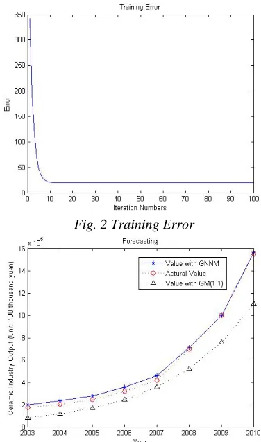
Fig. 2 Training Error

Fig. 3 Curve of Forecasting with Different Models

From Tables Ⅱ-Ⅳ it can be seen that the relative error of GM(1,1) is about 8 times of GNNM, posterior ratio and small error probability of GNNM are better than of GM(1,1), and GNNM gets quite satisfactory forecasting result. Where, posterior ratio of GNNM decreases greatly, which means that the error focused on the small-scale and achieves higher precise prediction. Fig. 2 shows GNNM converges fast and the network gets optimization quickly. In Fig. 3, the forecasting curve of GNNM is more close to the actual curve than the curve of GM(1,1), especially the forecasted value after 2008. This shows GNNM has the better forecasting effectiveness and accuracy.

5.

This paper discusses the modeling idea and the key steps of the grey neural network model about the ceramic industrial output forecasting. This model is applied to forecast in Matlab 7, and good result is obtained. The grey neural network model is

built by combining grey model and neural network model, which expands the application scope of GM(1,1) and improves the forecasting precision. In addition, the parameters of the grey neural network model influence the forecasting results greatly. In the future research, genetic algorithm can be used to optimize the parameters, which make prediction results more realistically reflect the actual situation.

ACKNOWLEDGMENT

This work is completed under the support of the National Key Technology R&D Program of China (No. 2013BAF02B01) and (No. 2012BAH25F02).

REFRENCES:

[1] DENG Ju-long. The Theory Book of Grey System [M].Wuhan: Huazhong University of Science and Technology Press, 1990.

using artificial neural networks and conceptual models [J].Journal of Hydrologic Engineering,2000,(4):156-161.

[3] WANGQ P. Application of BP NN for forecast of Chinese grain output [J]. Forecasting 2002, 21(3): 79-80.

[4] Zhou Zhi-hua, Cao Cun-geng. Application of Neural Network [M]. Beijing: Tsinghua University Press. 2004.

[5] Liu Guo-bi. Grain Forecasting Based on Gray Neural Network [J]. Journal of Anhui Agri. Sci. 2009, 37(26): 12362-12363.

[6] Wu Long-xiao, Hou Zhi-jian, Tai Neng-ling. Application of grey neural network model GNNM(1,1) in city electricity demand forecasting [J]. Electric Power, 2005, 38(2): 46-48

[7] Niu Dongxiao, Jia Jianrong. Application of Improved GM(1,1)Model in Load Forecasting [J]. Electric Power Science and Engineering. 2008, 24(4): 28-30.

[8] ZHOU Rui2ping. Application of the Grey Model to Forecasting Scale of Urban Population [J]. Journal of Inner Mongolia Normal University (Natural Science Edition). 2005, 34(1): 81-83

[9] Tian Ying. The GM(1,1) Model for Predicting Stock Market Based on Grey Theory [J]. Mathematics in Practice and Theory. 2001, 31(5): 523-524.