SRC RR 124 pdf

May 10, 1994

SRC

Research

Report

124

A Block-sorting Lossless

Data Compression Algorithm

M. Burrows and D.J. Wheeler

d i g i t a l

Systems Research Center

Systems Research Center

The charter of SRC is to advance both the state of knowledge and the state of the art in computer systems. From our establishment in 1984, we have performed basic and applied research to support Digital’s business objectives. Our current work includes exploring distributed personal computing on multiple platforms, network-ing, programming technology, system modelling and management techniques, and selected applications.

Our strategy is to test the technical and practical value of our ideas by building hardware and software prototypes and using them as daily tools. Interesting systems are too complex to be evaluated solely in the abstract; extended use allows us to investigate their properties in depth. This experience is useful in the short term in refining our designs, and invaluable in the long term in advancing our knowledge. Most of the major advances in information systems have come through this strategy, including personal computing, distributed systems, and the Internet.

We also perform complementary work of a more mathematical flavor. Some of it is in established fields of theoretical computer science, such as the analysis of algorithms, computational geometry, and logics of programming. Other work explores new ground motivated by problems that arise in our systems research. We have a strong commitment to communicating our results; exposing and testing our ideas in the research and development communities leads to improved un-derstanding. Our research report series supplements publication in professional journals and conferences. We seek users for our prototype systems among those with whom we have common interests, and we encourage collaboration with uni-versity researchers.

A Block-sorting Lossless

Data Compression Algorithm

M. Burrows and D.J. Wheeler

David Wheeler is a Professor of Computer Science at the University of Cambridge, U.K. His electronic mail address is: [email protected]

c

Digital Equipment Corporation 1994.

Authors’ abstract

We describe a block-sorting, lossless data compression algorithm, and our imple-mentation of that algorithm. We compare the performance of our impleimple-mentation with widely available data compressors running on the same hardware.

The algorithm works by applying a reversible transformation to a block of input text. The transformation does not itself compress the data, but reorders it to make it easy to compress with simple algorithms such as move-to-front coding.

Contents

1 Introduction 1

2 The reversible transformation 2

3 Why the transformed string compresses well 5

4 An efficient implementation 8

4.1 Compression : : : : : : : : : : : : : : : : : : : : : : : : : : : : 8 4.2 Decompression: : : : : : : : : : : : : : : : : : : : : : : : : : : 12

5 Algorithm variants 13

6 Performance of implementation 15

1

Introduction

The most widely used data compression algorithms are based on the sequential data compressors of Lempel and Ziv [1, 2]. Statistical modelling techniques may produce superior compression [3], but are significantly slower.

In this paper, we present a technique that achieves compression within a percent or so of that achieved by statistical modelling techniques, but at speeds comparable to those of algorithms based on Lempel and Ziv’s.

Our algorithm does not process its input sequentially, but instead processes a block of text as a single unit. The idea is to apply a reversible transformation to a block of text to form a new block that contains the same characters, but is easier to compress by simple compression algorithms. The transformation tends to group characters together so that the probability of finding a character close to another instance of the same character is increased substantially. Text of this kind can easily be compressed with fast locally-adaptive algorithms, such as move-to-front coding [4] in combination with Huffman or arithmetic coding.

Briefly, our algorithm transforms a string S of N characters by forming the N rotations (cyclic shifts) of S, sorting them lexicographically, and extracting the last character of each of the rotations. A string L is formed from these characters, where the ith character of L is the last character of the ith sorted rotation. In addition to

L, the algorithm computes the index I of the original string S in the sorted list of

rotations. Surprisingly, there is an efficient algorithm to compute the original string

S given only L and I .

The sorting operation brings together rotations with the same initial characters. Since the initial characters of the rotations are adjacent to the final characters, consecutive characters in L are adjacent to similar strings in S. If the context of a character is a good predictor for the character, L will be easy to compress with a simple locally-adaptive compression algorithm.

In the following sections, we describe the transformation in more detail, and show that it can be inverted. We explain more carefully why this transformation tends to group characters to allow a simple compression algorithm to work more effectively. We then describe efficient techniques for implementing the transfor-mation and its inverse, allowing this algorithm to be competitive in speed with Lempel-Ziv-based algorithms, but achieving better compression. Finally, we give the performance of our implementation of this algorithm, and compare it with well-known compression programmes.

2

The reversible transformation

This section describes two sub-algorithms. Algorithm C performs the reversible transformation that we apply to a block of text before compressing it, and Algorithm D performs the inverse operation. A later section suggests a method for compressing the transformed block of text.

In the description below, we treat strings as vectors whose elements are char-acters.

Algorithm C: Compression transformation

This algorithm takes as input a string S of N characters S[0]; : : : ;S[N 1] selected from an ordered alphabet X of characters. To illustrate the technique, we also give a running example, using the string S D ‘abraca’, N D 6, and the alphabet

X D f0_a0;0_b0;0_c0;0_r0_g.

C1. [sort rotations]

Form a conceptual N ð N matrix M whose elements are characters, and

whose rows are the rotations (cyclic shifts) of S, sorted in lexicographical order. At least one of the rows of M contains the original string S. Let I be the index of the first such row, numbering from zero.

In our example, the index I D1 and the matrix M is

row

0 aabrac

1 abraca

2 acaabr

3 bracaa

4 caabra

5 racaab

C2. [find last characters of rotations]

Let the string L be the last column of M, with characters L[0]; : : : ;L[N 1] (equal to M[0;N 1]; : : : ;M[N 1;N 1]). The output of the transfor-mation is the pair.L;I/.

In our example, LD‘caraab’ and I D1 (from step C1).

Algorithm D: Decompression transformation

We use the example and notation introduced in Algorithm C. Algorithm D uses the output.L;I/of Algorithm C to reconstruct its input, the string S of length N .

D1. [find first characters of rotations]

This step calculates the first column F of the matrix M of Algorithm C. This is done by sorting the characters of L to form F. We observe that any column of the matrix M is a permutation of the original string S. Thus, L and F are both permutations of S, and therefore of one another. Furthermore, because the rows of M are sorted, and F is the first column of M, the characters in F are also sorted.

In our example, F D‘aaabcr’. D2. [build list of predecessor characters]

To assist our explanation, we describe this step in terms of the contents of the matrix M. The reader should remember that the complete matrix is not available to the decompressor; only the strings F, L, and the index I (from the input) are needed by this step.

Consider the rows of the matrix M that start with some given character ch. Algorithm C ensured that the rows of matrix M are sorted lexicographically, so the rows that start with ch are ordered lexicographically.

We define the matrix M0_{formed by rotating each row of M one character to}

the right, so for each iD0; : : : ;N 1, and each j D0; : : : ;N 1,

M0_{[i; j ]D M[i; .j 1/mod N ]}

In our example, M and M0_are:

row M M0

0 aabrac caabra

1 abraca aabrac

2 acaabr racaab

3 bracaa abraca

4 caabra acaabr

5 racaab bracaa

Like M, each row of M0 _{is a rotation of S, and for each row of M there is}

of M0 _{are sorted lexicographically starting with their second character. So,}

if we consider only those rows in M0 _{that start with a character ch, they}

must appear in lexicographical order relative to one another; they have been sorted lexicographically starting with their second characters, and their first characters are all the same and so do not affect the sort order. Therefore, for any given character ch, the rows in M that begin with ch appear in the same

order as the rows in M0_{that begin with ch.}

In our example, this is demonstrated by the rows that begin with ‘a’. The rows ‘aabrac’, ‘abraca’, and ‘acaabr’ are rows 0, 1, 2 in M and correspond to rows 1, 3, 4 in M0_.

Using F and L, the first columns of M and M0 _{respectively, we calculate}

a vector T that indicates the correspondence between the rows of the two matrices, in the sense that for each j D0; : : : ;N 1, row j of M0_corresponds

to row T [ j ] of M.

If L[ j ] is the kth instance of ch in L, then T [ j ] D i where F[i] is the kth

instance of ch in F. Note that T represents a one-to-one correspondence between elements of F and elements of L, and F[T [ j ]]D L[ j ].

In our example, T is: (4 0 5 1 2 3).

D3. [form output S]

Now, for each i D 0; : : : ;N 1, the characters L[i] and F[i] are the last and first characters of the row i of M. Since each row is a rotation of

S, the character L[i] cyclicly precedes the character F[i] in S. From the

construction of T , we have F[T [ j ]]D L[ j ]. Substituting i DT [ j ], we have L[T [ j ]] cyclicly precedes L[ j ] in S.

The index I is defined by Algorithm C such that row I of M is S. Thus, the last character of S is L[I ]. We use the vector T to give the predecessors of each character:

for each i D0; : : : ;N 1: S[N 1 i]DL[Ti_{[I ]].}

where T0_{[x ]}

Dx , and TiC1_{[x ]}

DT [Ti_{[x ]]. This yields S, the original input}

to the compressor.

In our example, SD‘abraca’.

We could have defined T so that the string S would be generated from front to back, rather than the other way around. The description above matches the pseudo-code given in Section 4.2.

The sequence Ti_{[I ] for i D0; : : : ;N 1 is not necessarily a permutation of}

the numbers 0; : : : ;N 1. If the original string S is of the form Zp _{for some}

substring Z and some p > 1, then the sequence Ti_{[I ] for i D0}; : : : ;_{N 1 will}

also be of the form Z0p _{for some subsequence Z}0_{. That is, the repetitions in S will}

be generated by visiting the same elements of T repeatedly. For example, if S D

‘cancan’, Z D‘can’ and pD2, the sequence Ti_{[I ] for iD0; : : : ;N 1 will be}

[2;4;0;2;4;0].

3

Why the transformed string compresses well

Algorithm C sorts the rotations of an input string S, and generates the string L consisting of the last character of each rotation.

To see why this might lead to effective compression, consider the effect on a single letter in a common word in a block of English text. We will use the example of the letter ‘t’ in the word ‘the’, and assume an input string containing many instances of ‘the’.

When the list of rotations of the input is sorted, all the rotations starting with ‘he ’ will sort together; a large proportion of them are likely to end in ‘t’. One region of the string L will therefore contain a disproportionately large number of ‘t’ characters, intermingled with other characters that can proceed ‘he ’ in English, such as space, ‘s’, ‘T’, and ‘S’.

The same argument can be applied to all characters in all words, so any localized region of the string L is likely to contain a large number of a few distinct characters. The overall effect is that the probability that given character ch will occur at a given point in L is very high if ch occurs near that point in L, and is low otherwise. This property is exactly the one needed for effective compression by a move-to-front coder [4], which encodes an instance of character ch by the count of distinct characters seen since the next previous occurrence of ch. When applied to the string L, the output of a move-to-front coder will be dominated by low numbers, which can be efficiently encoded with a Huffman or arithmetic coder.

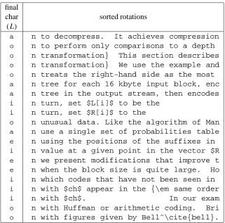
Figure 1 shows an example of the algorithm at work. Each line is the first few characters and final character of a rotation of a version of this document. Note the grouping of similar characters in the column of final characters.

final

char sorted rotations (L)

a n to decompress. It achieves compression

o n to perform only comparisons to a depth

o n transformation} This section describes

o n transformation} We use the example and

o n treats the right-hand side as the most

a n tree for each 16 kbyte input block, enc

a n tree in the output stream, then encodes

i n turn, set $L[i]$ to be the

i n turn, set $R[i]$ to the

o n unusual data. Like the algorithm of Man

a n use a single set of probabilities table

e n using the positions of the suffixes in

i n value at a given point in the vector $R

e n we present modifications that improve t

e n when the block size is quite large. Ho

i n which codes that have not been seen in

i n with $ch$ appear in the {\em same order

i n with $ch$. In our exam

o n with Huffman or arithmetic coding. Bri

o n with figures given by Bell˜\cite{bell}.

Figure 1: Example of sorted rotations. Twenty consecutive rotations from the sorted list of rotations of a version of this paper are shown, together with the final character of each rotation.

Algorithm M: Move-to-front coding

This algorithm encodes the output.L;I/ of Algorithm C, where L is a string of length N and I is an index. It encodes L using a move-to-front algorithm and a Huffman or arithmetic coder.

The running example of Algorithm C is continued here.

M1. [move-to-front coding]

This step encodes each of the characters in L by applying the move-to-front technique to the individual characters. We define a vector of integers

R[0]; : : : ;R[N 1], which are the codes for the characters L[0]; : : : ;L[N

1].

Initialize a list Y of characters to contain each character in the alphabet X exactly once.

For each i D 0; : : : ;N 1 in turn, set R[i] to the number of characters preceding character L[i] in the list Y, then move character L[i] to the front of Y.

Taking Y D [0

a0;0b0;0c0;0r0] initially, and L D‘caraab’, we compute the vector R: (2 1 3 1 0 3).

M2. [encode]

Apply Huffman or arithmetic coding to the elements of R, treating each element as a separate token to be coded. Any coding technique can be applied as long as the decompressor can perform the inverse operation. Call the output of this coding process OUT. The output of Algorithm C is the pair

.OUT;I/where I is the value computed in step C1.

Algorithm W: Move-to-front decoding

This algorithm is the inverse of Algorithm M. It computes the pair.L;I/from the pair.OUT;I/.

We assume that the initial value of the list Y used in step M1 is available to the decompressor, and that the coding scheme used in step M2 has an inverse operation.

W1. [decode]

Decode the coded stream OUT using the inverse of the coding scheme used in step M2. The result is a vector R of N integers.

W2. [inverse move-to-front coding]

The goal of this step is to calculate a string L of N characters, given the move-to-front codes R[0]; : : : ;R[N 1].

Initialize a list Y of characters to contain the characters of the alphabet X in the same order as in step M1.

For each i D 0; : : : ;N 1 in turn, set L[i] to be the character at position

R[i] in list Y (numbering from 0), then move that character to the front of Y.

The resulting string L is the last column of matrix M of Algorithm C. The output of this algorithm is the pair.L;I/, which is the input to Algorithm D. Taking Y D [0_a0;0_b0;0_c0;0_r0_{] initially (as in Algorithm M), we compute the}

string LD‘caraab’.

4

An efficient implementation

Efficient implementations of move-to-front, Huffman, and arithmetic coding are well known. Here we concentrate on the unusual steps in Algorithms C and D.

4.1

Compression

The most important factor in compression speed is the time taken to sort the rotations of the input block. A simple application of quicksort requires little additional space (one word per character), and works fairly well on most input data. However, its worst-case performance is poor.

A faster way to implement Algorithm C is to reduce the problem of sorting the rotations to the problem of sorting the suffixes of a related string.

To compress a string S, first form the string S0_{, which is the concatenation of S}

with EOF, a new character that does not appear in S. Now apply Algorithm C to S0_.

Because EOF is different from all other characters in S0_{, the suffixes of S}0_{sort in the}

same order as the rotations of S0_{. Hence, to sort the rotations, it suffices to sort the}

suffixes of S0_{. This can be done in linear time and space by building a suffix tree,}

which then can be walked in lexicographical order to recover the sorted suffixes. We used McCreight’s suffix tree construction algorithm [5] in an implementation of Algorithm C. Its performance is within 40% of the fastest technique we have found when operating on text files. Unfortunately, suffix tree algorithms need space for more than four machine words per input character.

Manber and Myers give a simple algorithm for sorting the suffixes of a string in O.N log N/time [6]. The algorithm they describe requires only two words per

input character. The algorithm works by sorting suffixes on their first i characters, then using the positions of the suffixes in the sorted array as the sort key for another sort on the first 2i characters. Unfortunately, the performance of their algorithm is significantly worse than the suffix tree approach.

The fastest scheme we have tried so far uses a variant of quicksort to generate the sorted list of suffixes. Its performance is significantly better than the suffix tree when operating on text, and it uses significantly less space. Unlike the suffix tree however, its performance can degrade considerably when operating on some types of data. Like the algorithm of Manber and Myers, our algorithm uses only two words per input character.

Algorithm Q: Fast quicksorting on suffixes

This algorithm sorts the suffixes of the string S, which contains N characters

S[0; : : : ;N 1]. The algorithm works by applying a modified version of quicksort to the suffixes of S.

First we present a simple version of the algorithm. Then we present modifica-tions that improve the speed and make bad performance less likely.

Q1. [form extended string]

Let k be the number of characters that fit in a machine word.

Form the string S0 _{from S by appending k additional EOF characters to S,}

where EOF does not appear in S.

Q2. [form array of words]

Initialize an array W of N words W[0; : : : ;N 1], such that W[i] contains the characters S0_{[i; : : : ;iCk 1] arranged so that integer comparisons on}

the words agree with lexicographic comparisons on the k-character strings. Packing characters into words has two benefits: It allows two prefixes to be compared k bytes at a time using aligned memory accesses, and it allows many slow cases to be eliminated (described in step Q7).

Q3. [form array of suffixes]

In this step we initialize an array V of N integers. If an element of V contains j , it represents the suffix of S0_{whose first character is S}0_{[ j ]. When}

the algorithm is complete, suffix V [i] will be the ith suffix in lexicographical order.

Q4. [radix sort]

Sort the elements of V , using the first two characters of each suffix as the sort key. This can be done efficiently using radix sort.

Q5. [iterate over each character in the alphabet]

For each character ch in the alphabet, perform steps Q6, Q7.

Once this iteration is complete, V represents the sorted suffixes of S, and the algorithm terminates.

Q6. [quicksort suffixes starting with ch]

For each character ch0_{in the alphabet: Apply quicksort to the elements of V}

starting with ch followed by ch0_{. In the implementation of quicksort, compare}

the elements of V by comparing the suffixes they represent by indexing into the array W. At each recursion step, keep track of the number of characters that have compared equal in the group, so that they need not be compared again.

All the suffixes starting with ch have now been sorted into their final positions in V .

Q7. [update sort keys]

For each element V [i] corresponding to a suffix starting with ch (that is, for which S[V [i]] Dch), set W[V [i]] to a value with ch in its high-order bits

(as before) and with i in its low-order bits (which step Q2 set to the k 1 characters following the initial ch). The new value of W[V [i]] sorts into the same position as the old value, but has the desirable property that it is distinct from all other values in W. This speeds up subsequent sorting operations, since comparisons with the new elements cannot compare equal.

This basic algorithm can be refined in a number of ways. An obvious improve-ment is to pick the character ch in step Q5 starting with the least common character in S, and proceeding to the most common. This allows the updates of step Q7 to have the greatest effect.

As described, the algorithm performs poorly when S contains many repeated substrings. We deal with this problem with two mechanisms.

The first mechanism handles strings of a single repeated character by replacing step Q6 with the following steps.

Q6a. [quicksort suffixes starting ch;ch0_{where ch6Dch}0_]

For each character ch0_{6Dch in the alphabet: Apply quicksort to the elements}

of V starting with ch followed by ch0_{. In the implementation of quicksort,}

compare the elements of V by comparing the suffixes they represent by indexing into the array W. At each recursion step, keep track of the number of characters that have compared equal in the group, so that they need not be compared again.

Q6b. [sort low suffixes starting ch;ch]

This step sorts the suffixes starting runs which would sort before an infinite string of ch characters. We observe that among such suffixes, long initial runs of character ch sort after shorter initial runs, and runs of equal length sort in the same order as the characters at the ends of the run. This ordering can be obtained with a simple loop over the suffixes, starting with the shortest. Let V[i] represent the lexicographically least suffix starting with ch. Let j be the lowest value such that suffix V [ j ] starts with ch;ch.

while not (i = j) do

if (V[i] > 0) and (S[V[i]-1] = ch) then V[j] := V[i]-1;

j := j + 1 end;

i := i + 1 end;

All the suffixes that start with ch;ch and that are lexicographically less than

an infinite sequence of ch characters are now sorted.

Q6c. [sort high suffixes starting ch;ch]

This step sorts the suffixes starting runs which would sort after an infinite string of ch characters. This step is very like step Q6b, but with the direction of the loop reversed.

Let V [i] represent the lexicographically greatest suffix starting with ch. Let

j be the highest value such that suffix V [ j ] starts with ch;ch.

while not (i = j) do

if (V[i] > 0) and (S[V[i]-1] = ch) then V[j] := V[i]-1;

j := j - 1 end;

i := i - 1 end;

All the suffixes that start with ch;ch and that are lexicographically greater

The second mechanism handles long strings of a repeated substring of more than one character. For such strings, we use a doubling technique similar to that used in Manber and Myers’ scheme. We limit our quicksort implementation to perform comparisons only to a depth D. We record where suffixes have been left unsorted with a bit in the corresponding elements of V .

Once steps Q1 to Q7 are complete, the elements of the array W indicate sorted positions up to Dðk characters, since each comparison compares k characters. If

unsorted portions of V remain, we simply sort them again, limiting the comparison depth to D as before. This time, each comparison compares Dðk characters, to

yield a list of suffixes sorted on their first D2_{ðk characters. We repeat this process}

until the entire string is sorted.

The combination of radix sort, a careful implementation of quicksort, and the mechanisms for dealing with repeated strings produce a sorting algorithm that is extremely fast on most inputs, and is quite unlikely to perform very badly on real input data.

We are currently investigating further variations of quicksort. The following approach seems promising. By applying the technique of Q6a–Q6c to all overlap-ping repeated strings, and by caching previously computed sort orders in a hash table, we can produce an algorithm that sorts the suffixes of a string in approxi-mately the same time as the modified algorithm Q, but using only 6 bytes of space per input character (4 bytes for a pointer, 1 byte for the input character itself, and 1 byte amortized space in the hash table). This approach has poor performance in the worst case, but bad cases seem to be rare in practice.

4.2

Decompression

Steps D1 and D2 can be accomplished efficiently with only two passes over the data, and one pass over the alphabet, as shown in the pseudo-code below. In the first pass, we construct two arrays: C[alphabet] and P[0; : : : ;N 1]. C[ch] is the total number of instances in L of characters preceding character ch in the alphabet.

P[i] is the number of instances of character L[i] in the prefix L[0; : : : ;i 1] of

L. In practice, this first pass could be combined with the move-to-front decoding

step. Given the arrays L, C, P, the array T defined in step D2 is given by: for each i D0; : : : ;N 1 : T [i]D P[i]CC[L[i]]

In a second pass over the data, we use the starting position I to complete Algorithm D to generate S.

Initially, all elements of C are zero, and the last column of matrix M is the vector

L[0; : : : ;N 1].

for i := 0 to N-1 do P[i] := C[L[i]];

C[L[i]] := C[L[i]] + 1 end;

Now C[ch] is the number of instances in L of character ch. The value P[i] is the number of instances of character L[i] in the prefix L[0; : : : ;i 1] of L.

sum := 0;

for ch := FIRST(alphabet) to LAST(alphabet) do sum := sum + C[ch];

C[ch] := sum - C[ch]; end;

Now C[ch] is the total number of instances in L of characters preceding ch in the alphabet.

i := I;

for j := N-1 downto 0 do S[j] := L[i];

i := P[i] + C[L[i]] end

The decompressed result is now S[0; : : : ;N 1].

5

Algorithm variants

In the example given in step C1, we treated the left-hand side of each rotation as the most significant when sorting. In fact, our implementation treats the right-hand side as the most significant, so that the decompressor will generate its output S from left to right using the code of Section 4.2. This choice has almost no effect on the compression achieved.

The algorithm can be modified to use a different coding scheme instead of move-to-front in step M1. Compression can improve slightly if move-to-front is replaced by a scheme in which codes that have not been seen in a very long time are moved only part-way to the front. We have not exploited this in our implementations.

Size CPU time/s Compressed bits/ File (bytes) compress decompress size (bytes) char bib 111261 1.6 0.3 28750 2.07 book1 768771 14.4 2.5 238989 2.49 book2 610856 10.9 1.8 162612 2.13 geo 102400 1.9 0.6 56974 4.45 news 377109 6.5 1.2 122175 2.59 obj1 21504 0.4 0.1 10694 3.98 obj2 246814 4.1 0.8 81337 2.64 paper1 53161 0.7 0.1 16965 2.55 paper2 82199 1.1 0.2 25832 2.51 pic 513216 5.4 1.2 53562 0.83 progc 39611 0.6 0.1 12786 2.58 progl 71646 1.1 0.2 16131 1.80 progp 49379 0.8 0.1 11043 1.79 trans 93695 1.6 0.2 18383 1.57 Total 3141622 51.1 9.4 856233

-Table 1: Results of compressing fourteen files of the Calgary Compression Corpus.

Block size bits/character (bytes) book1 Hector corpus

1k 4.34 4.35 4k 3.86 3.83 16k 3.43 3.39 64k 3.00 2.98 256k 2.68 2.65 750k 2.49

-1M - 2.43

4M - 2.26

16M - 2.13

64M - 2.04

103M - 2.01

Table 2: The effect of varying block size ( N ) on compression ofbook1from the Calgary Compression Corpus and of the entire Hector corpus.

6

Performance of implementation

In Table 1 we give the results of compressing the fourteen commonly used files of the Calgary Compression Corpus [7] with our algorithm. Comparison of these figures with those given by Bell, Witten and Cleary [3] indicate that our algorithm does well on non-text inputs as well as text inputs.

Our implementation of Algorithm C uses the techniques described in Sec-tion 4.1, and a simple move-to-front coder. In each case, the block size N is the length of the file being compressed.

We compress the output of the move-to-front coder with a modified Huffman coder that uses the technique described in Section 5. Our coder calculates new Huffman trees for each 16 kbyte input block, rather than computing one tree for its whole input.

In Table 1, compression effectiveness is expressed as output bits per input character. The CPU time measurements were made on a DECstation 5000/200, which has a MIPS R3000 processor clocked at 25MHz with a 64 kbyte cache. CPU time is given rather than elapsed time so the time spent performing I/O is excluded. In Table 2, we show the variation of compression effectiveness with input block size for two inputs. The first input is the filebook1from the Calgary Compression Corpus. The second is the entire Hector corpus [8], which consists of a little over 100 MBytes of modern English text. The table shows that compression improves with increasing block size, even when the block size is quite large. However, increasing the block size above a few tens of millions of characters has only a small effect.

If the block size were increased indefinitely, we expect that the algorithm would not approach the theoretical optimum compression because our simple byte-wise move-to-front coder introduces some loss. A better coding scheme might achieve optimum compression asymptotically, but this is not likely to be of great practical importance.

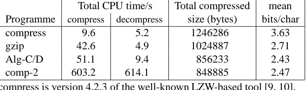
Comparison with other compression programmes

Total CPU time/s Total compressed mean Programme compress decompress size (bytes) bits/char compress 9.6 5.2 1246286 3.63 gzip 42.6 4.9 1024887 2.71 Alg-C/D 51.1 9.4 856233 2.43 comp-2 603.2 614.1 848885 2.47 compress is version 4.2.3 of the well-known LZW-based tool [9, 10]. gzip is version 1.2.4 of Gailly’s LZ77-based tool [1, 11].

Alg-C/D is Algorithms C and D, with our back-end Huffman coder. comp-2 is Nelson’s comp-2 coder, limited to a fourth-order model [12].

Table 3: Comparison with other compression programmes.

7

Conclusions

We have described a compression technique that works by applying a reversible transformation to a block of text to make redundancy in the input more accessible to simple coding schemes. Our algorithm is general-purpose, in that it does well on both text and non-text inputs. The transformation uses sorting to group characters together based on their contexts; this technique makes use of the context on only one side of each character.

To achieve good compression, input blocks of several thousand characters are needed. The effectiveness of the algorithm continues to improve with increasing block size at least up to blocks of several million characters.

Our algorithm achieves compression comparable with good statistical mod-ellers, yet is closer in speed to coders based on the algorithms of Lempel and Ziv. Like Lempel and Ziv’s algorithms, our algorithm decompresses faster than it compresses.

Acknowledgements

We would like to thank Andrei Broder, Cynthia Hibbard, Greg Nelson, and Jim Saxe for their suggestions on the algorithms and the paper.

References

[1] J. Ziv and A. Lempel. A universal algorithm for sequential data compression. IEEE Transactions on Information Theory. Vol. IT-23, No. 3, May 1977, pp. 337–343.

[2] J. Ziv and A. Lempel. Compression of individual sequences via variable rate coding. IEEE Transactions on Information Theory. Vol. IT-24, No. 5, September 1978, pp. 530–535.

[3] T. Bell, I. H. Witten, and J.G. Cleary. Modeling for text compression. ACM Computing Surveys, Vol. 21, No. 4, December 1989, pp. 557–589.

[4] J.L. Bentley, D.D. Sleator, R.E. Tarjan, and V.K. Wei. A locally adaptive data compression algorithm. Communications of the ACM, Vol. 29, No. 4, April 1986, pp. 320–330.

[5] E.M. McCreight. A space economical suffix tree construction algorithm. Jour-nal of the ACM, Vol. 32, No. 2, April 1976, pp. 262–272.

[6] U. Manber and E. W. Myers, Suffix arrays: A new method for on-line string searches. SIAM Journal on Computing, Volume 22, No. 5, October 1993, pp. 935-948.

[7] I. H. Witten and T. Bell. The Calgary/Canterbury text compression cor-pus. Anonymous ftp fromftp.cpsc.ucalgary.ca: /pub/text.com-pression.corpus/text.compression.corpus.tar.Z

[8] L. Glassman, D. Grinberg, C. Hibbard, J. Meehan, L. Guarino Reid, and M-C. van Leunen. Hector: Connecting Words with Definitions. Proceedings of the 8th Annual Conference of the UW Centre for the New Oxford English Dictionary and Text Research, Waterloo, Canada, October, 1992. pp. 37– 73. Also available as Research Report 92a, Digital Equipment Corporation Systems Research Center, 130 Lytton Ave, Palo Alto, CA. 94301.

[9] T.A. Welch. A technique for high performance data compression. IEEE Com-puter, Vol. 17, No. 6, June 1984, pp. 8–19.

[10] Peter Jannesen et al. Compress, Version 4.2.3. Posted to the Internet news-groupcomp.sources.reviewed, 28th August, 1992. Anonymous ftp from

[11] J. Gailly et al. Gzip, Version 1.2.4. Anonymous ftp fromprep.ai.mit.edu: /pub/gnu/gzip-1.2.4.tar.gz

[12] Mark Nelson. Arithmetic coding and statistical modeling. Dr. Dobbs Journal. February, 1991. Anonymous ftp from wuarchive.wustl.edu: /mir-rors/msdos/ddjmag/ddj9102.zip