4251
CONFORMABLE DECOMPOSITION METHOD FOR
TIME-SPACE FRACTIONAL INTERMEDIATE SCALAR
TRANSPORTATION MODEL
S.O. EDEKI1*, G. O. AKINLABI2, R. M. JENA3, O.P. OGUNDILE4, S. CHAKRAVERTY5
1Department of Mathematics, Covenant University, Canaanland, Ota, Nigeria 2Department of Mathematics, National Institute of Technology, Rourkela, India
E-mail: 1*[email protected], 2[email protected], 3[email protected], 4[email protected], 5sne [email protected]
ABSTRACT
This paper considers the analytical solutions of a time-space fractional intermediate scalar transportation model via the application of Conformable Decomposition Algorithm. The method is a blend of Adomian Decomposition coupled with fractional derivative defined in conformable sense; herein referred to as CADM. Illustrative examples (cases) are considered in order to clarify the effectiveness of the proposed method, and the solutions are presented in infinite series form with high level of convergence to the exact form of solution.
Keywords: Advection-Dispersion Model, Adomian Decomposition Method, Fractional Calculus, Conformable Derivative
1. INTRODUCTION
The Advection Dispersion equation (ADE) also known as Advection diffusion equation is a well-known method in applied engineering and physics. It is mostly applied in the area of transportation modelling. This equation can be used to solve and analyse time and space differences in a particle activity [1-2]. Mostly, the results of this particular equation equipped with boundary conditions require the application of numerical methods. Meanwhile, the corresponding model has been investigated by many scholars using the stochastic, analytic and numerical approaches [2-4]. It is a generally accepted fact that in life fluids moves through the combined effect of advection and diffusion motion. The coupling of Fractional Complex Transform (FCT) with modified version of differential transform method has been applied for exact solutions of time fractional ADE [5].
Several authors have also examined the governing equation that is classically and traditionally used to model the dissolve solutes, mainly for this equation to be well positioned some important assumptions must be valid [6-7].
ADE has been used to illustrate a dynamical system, for example, a groundwater pollution model, coupled with a generalised analytical solution for one-dimensional solute transport in countable spatial domain. This method can also take two-dimensional form, which can be approximated but it poses a lot of challenges for the researcher and it is equally very important to consider. This is in recent time has actually motivated a lot of strong research work [8-9].
Over the years, many scholars have developed Fractional Advection-Dispersion Equation (FADE) from the advection-dispersion equation, some solved a notable number of problems using the finite difference approach, while some considered an open channel shallow water, and some set of scholars have also combined ADE with KDV which was solved numerically by the use of (FCCS) scheme and their results proffered significant solutions [ 9-16].
4252
2
1 2 2
0
,
0
,0
w
w
w
u
u
w
w
(1)
where
w
,
w
represents the dissolved concentration,u
1and
u
2 are Darcy velocity and dispersion coefficient respectively.Sayed and Behiry and Raslan [17] extended (1) to time-fractional form:
,
,
, ,
0,
0,1
,
1
2
,0
.
x
x
h x
D h x
x
t
h x
e
(2) In their work [17], they used (2) to describe the intermediate process that occurs between advection and dispersion using fractional derivative in the Caputo sense with the aid of Adomian's decomposition method. In this paper, (1) and (2) will be considered for extension in the direction of time-space fractional derivative as regards conformable view of fractional derivative. Hence, time-space fractional intermediate scalar transportation model of the form:
0,
,
, ,
0,
0,1
,
1
2
,
1,2 ,
0,1
,0
.
t x
D h x t
D h x t t
x
h x
h
(3) In considering the solutions of classical, and fractional differential models, various solution methods include the views of [18-31]. Here, Adomian Decomposition Method coupled with fractional derivative defined in conformable sense (CADM) is mainly applied for the first time, regarding analytical solution of a time-space fractional intermediate scalar transportation model. The structure of the remaining parts of the paper will be as follows, we have in section 2: a brief notion of conformable differential operator and its properties, section 3 is on the proposed solution method (CADM), section 4 contains the application while section 5 is on concluding remarks.
2. BASIC NOTIONS OF CONFORMABLE
DIFFERENTIAL OPERATORS [32-35]
Definition (1): For a function
h
: 0,
, the conformable derivative ofh
of order
0,
is defined as:
1
0lim
h t
t
h t
,
0.
C h t
t
. (4)
2.1 Properties of Conformable Differential Operators CDOs
Let
h h t
,h
1
h t
1
andh
2
h t
2
bedifferentiable
functions att
0
for
. Then the following hold:(P1):
1 1
1 1 2 2 2 2
1 2
,
,
,
.
C h
C
h
h
C h
(P2):
C h
0,
,
.
(P3):
C h h
1 2
h C h
1
2
h C h
2
1.
(P4): 1 2
1 1
2 22 2
.
h C h
h C h
h
C
h
h
(P5):
C t
t
,
,
.
(P6):
C h t
t h t
1
,
h t
dh
.
dt
(P7): Suppose further that
h t
is ann
-times differentiable function att
, then:
,
1 ,
t
h
t
C h t
n n
where
denotes the smallest integer such that4253
3. THE CONFORMABLE SENSE OF THE
DECOMPOSITION METHOD [32-35]
Consider a general fractional (nonlinear) partial differential equation (NLFDE) of the form:
,
,
,
,
L h x t
R h x t
N h x t
q x t
(5) where
L
denotes a linear operator based on conformable derivative of order
, with respect tot
, such that
n n
,
1
,R
is the remaining part of the linear conformable differential operator,N
denotes the nonlinear operator, whileq x t
,
is the associated non-homogeneous part (source term).Suppose
L
C
is invertible such that
1L
exists, then (5) becomes:
,
,
,
,
C h x t
R h x t
q x t
N h x t
. (6)
Hence, by the differential property of the conformable derivative (P7), we have:
,
, .
,
t
h
t
R h x t
q x t
N h x t
(7)
,
,
,
,
q x t
h x t
R h x t
t
t
N h x t
. (8) The inverse operator is defined as follows:
1 1
1 1 1
1
.
n t n no o o
L
d d
d
(9)So, applying (9) to both sides of (8) gives:
1 1,
,
,
.
,
q x t
h x t
R h x t
L
t
L
t
N h x t
(10)
1 1,0
,
,
,
,
h x
L q x t
h x t
L
R h x t
N h x t
. (11) For the decomposition of the solution, we write:
0
,
n,
n
h x t
h x t
(12)while the nonlinear term with the Adomian polynomials
A
n is defined as:
0
,
n.
n
N h x t
A
(13)and
A
n (the Adomian polynomials) is given as:0 0
1
!
n n
i
n n i
i
A
N
h
n
. (14)Thus, using (12-14) in (10) gives:
1 0 1 0 0,0
,
,
,
.
t n n n n t n nh x
L
q x t
R
h x t
h x t
L
N
A
(15)Hence, in recursive relation, we have:
1 0 1 1,0
,
,
0.
tn t n n
h
h x
L
q x t
h
L
R h
A
n
4254 and
h x t
,
is therefore confirmed as:
0
,
lim
nn n
h x t
h
(17)4. APPLICATIONS AND ILLUSTRATIVE EXAMPLES
Here, the CADM as proposed above will be applied to some time-space fractional advection-dispersion model (TSFADM) as follows:
Example 1: Consider the following form of TSFADM:
,
,
, ,
0,
0,1
,
1
2
,0
.
t x
x
D h x t
D h x t t
x
h x
e
(18) Procedure: LetD h
t
C h
be applied to (18). Thus,
,
,
, 0
.
x x
C h x t
D h x t
h x
e
, (19)By (P6), we have:
1
,
, .
x
h x t
t
D h x t
t
(20)So, operating 1
1
0
1
t
L
d
on both sides of (20) gives:
,
, 0
1
,
.
x
h x t
h x
L
D h x t
(21) By decomposingh x t
,
, we have:
0 1 0,
,0
,
.
n n n nh x t
h x
L
h x t
x
(22) Thus,
0 1 1,0
,
,
0.
n nh
h x
h
L
h x t
x
n
(23)Therefore, the recursive relation in (23) yields:
0 1 1 0 1 2 1 1 3 2 1 4 3 1 1,0
k kh
h x
h
L
h
x
h
L
h
x
h
L
h
x
h
L
h
x
h
L
h
x
(24)whence, for:
h
0
e
x, the following are obtained:
0 1 1 0 2 2 1 2 2 1 3 3 1 3 3 2 4 4 1 4 4 3 1 1,0
1
,
1
,
2!
1
,
3!
1
,
4!
1
,
!
rx x x x x k k k x k kh
h x
e
t
h
L
h
e
x
t
h
L
h
e
x
t
h
L
h
e
x
t
h
L
h
e
x
t
h
L
h
e
x
k
0 .
k N
4255 Hence,
0 0
,
1
.
!
n
k k
n
n x
k n
n n
t
h x t
h
e
n
(26)
0
0
,
1
!
1
1
.
!
2
n n
x n
n
n
n n x
n
t
h x t
e
n
t
e
n
(27)
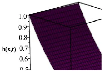
Equation (27) yields the solution of (18) in analytical form corresponding to the time-space fractional advection-dispersion.
In what follows, we present the graphical views of the solution for different values associated with the model parameters. This is considered for integer and fractional orders as contained in Fig. 1 through Fig. 8.
If
1, and
1
(for integral order, not fractional order) then the Eq. (1) reduces to pure advection equation (one may see Eq. (16) of refer [17]) and for this Eq. (1) reduces to
x
t
e
x th
,
. (28)If
2, and
1
(for integral order, not fractional order ) then the Eq. (1) reduces to pure diffusion equation (one may see Eq. (17) of refer [17]) and for this Eq. (1) reduces to
h
x
,
t
e
xt. (29) [image:5.612.324.527.123.264.2]Figure 1. Plot of (27) at
1, &
1
[image:5.612.318.521.318.447.2]Figure 2. Plot of (27):
1,
2,
0.01.
Figure 3. Plot of (27) at
0.2,&
1.
4256
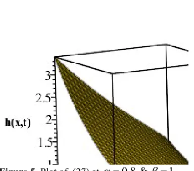
Figure 5. Plot of (27) at
0.8,&
1.
Figure 6. Plot of (27) at
1
,
1
.
2
and01
.
0
.Figure 7. Plot of (27) at
0.5,
1.8,
0.01.
Note: Figures 1 through 7, show the graphical representations of the solutions at different values of the associated parameters. All these are obtained via the maple software. It is remarked that the approach can be linked to other transformational techniques such as cosine
transformation, slant transformation, Adomian decomposition, Haar transformation, Dobeshi-4 transform, Hankel transformation, hadamard transformation and so on with various aspect of applications including textural images, high way transportation, etc [36-40].
5. CONCLUDING REMARKS
In this paper, Adomian Conformable Decomposition Method (CADM) has been successfully implemented for the solutions of a time-space fractional intermediate scalar transportation model as posed by Sayed and Behiry and Raslan [17]. The results from the Illustrative applications considered showed the efficiency and effectiveness of the proposed technique, while the solutions expressed in infinite series form converged to their exact form of solution. The effects of the time and space fractional parameters were considered for the cases of pure advection and pure diffusion. The considered algorithm or proposed solution method has special feature with ease in overcoming the tedious nature posed by space-fractional models unlike the time-fractional models. Hence, our recommendation of this approach.
CONFLICT OF INTERESTS
No conflict of interest is declared by the authors.
ACKNOWLEDGEMENTS
The authors1 appreciate the support from Covenant
University, and the effort of the anonymous reviewers
.
REFERENCES
[1] J M. Ramirez, E. A. “Thomann and E. C. Waymire” Statistical Science, 28(4), 2013, 487–509.
[2] C. Ancey, P. Bohorquez, and J. Heyman,
“Stochastic interpretation of the advection-diffusion equation and its relevance to bed
load transport”, J. Geophys. Res. Earth Surf.,
120, 2015, doi: 10.1002/2014JF003421.
4257 [4] K.H. Lai, C.W Liu, C.P. Liang, J.S. Chen, and
B.R. Sie,.”A novel method for analytically solving a radial advection-dispersion equation”, J. Hydrol., 542, 2016, 532-540. [5] S. O. Edeki, G. O. Akinlabi, and C. E. Odo,
“Fractional Complex Transform for the Solution of Time-Fractional Advection-Diffusion Model”, International Journal of Circuits, Systems and Signal Processing, 11, 2017, 425-432
[6] M. Massabo, R. Cianci, and O. Paladino . “An Analytical Solution of the Advection Dispersion Equation in a Bounded Domain and Its Application to Laboratory Experiments”, Journal of Applied Mathematics, 2011, 14 pages doi:10.1155/2011/493014
[7] D.A. Benson, “The Fractional Advection--Dispersion Equation: Development and Application. PhD Dissertation”, 1998.
[8] A. Atangana, “A generalized advection dispersion equation”, J. Earth Syst. Sci. 123 (1), 2014, 101-108.
[9] J. S. Chen and C.W. Liu., “Generalized analytical solution for advection-dispersion equation in finite spatial domain with arbitrary time-dependent inlet boundary condition”,
Hydrol. Earth Syst. Sci., 15, 2011, 2471–2479. [10] A. Chatterjee,. and M.K. Singh, “Two-dimensional advection-dispersion equation with depth- dependent variable source concentration”, Pollution, 4(1), 2018, 1-8. [11] F. Cristovao and K. Bryan, “Numerical
solution of the advection-dispersion-reaction equation under transient hydraulic conditions”, Conference proceeding, 2012.
[12] S, Rina, D A. Benson, M. M. Meerschaert, and S. W. Wheatcraft, “Eulerian derivation of the fractional advection–dispersion equation”,
Journal of Contaminant Hydrology, 48, 2001, 69–88.
[13] A.D. Benson, S.W. Wheatcraft, and M.M. Meerschaert, “Application of a fractional advection-dispersion equation”, Water Resour. Res., 36 (6), 2000, 1403-1412.
[14] S.G. Ahmed, “A Numerical Algorithm for Solving Advection-Diffusion Equation with Constant and Variable Coefficients”, The Open Numerical Methods Journal, 4, 2012, 1-7.
[15] M. A. Fauzi and F A. Zaky, “1-Dimensional Advection-Diffusion Finite Difference Model Due to a Flow under Propagating Solitary Wave” 4th International Conference on
Future Environment and Energy IPCBEE vol. 61, 2014.
[16] A.G. Hunt, and B. Ghanbarian, “Percolation theory for solute transport in porous media: Geochemistry, geomorphology, and carbon cycling” Water Resour. Res., 52(9), 2016, 7444-7459.
[17] A.M.A. El-Sayed, S.H. Behiry, W.E. Raslan, “Adomian's decomposition method for solving an intermediate fractional advection-dispersion equation”, Computers and Mathematics with Applications , 59, 2010, 1759-1765.
[18] G. Adomian, “Solving Frontier Problems of Physics: The Decomposition Method”, Kluwer Academic Publishers, Boston, 1994.
[19] R. Jena, S. Chakraverty, “Residual power series method for solving time-fractional model of vibration equation of large membranes” Journal of Applied and Computational Mechanics, 2018; doi: 10.22055/jacm.2018.26668.1347
[20] O. González-Gaxiola, S. O. Edeki, O.O. Ugbebor, and J.R. de Chávez, “Solving the Ivancevic Pricing Model Using the He's Frequency Amplitude Formulation” European Journal of Pure and Applied Mathematics, 10
(4), 2017, 631-637.
[21] S. O. Edeki, O.O. Ugbebor, and E. A. Owoloko, “On a Dividend-Paying Stock Options Pricing Model (SOPM) Using Constant Elasticity of Variance Stochastic Dynamics” International Journal of Pure and Applied Mathematics, 106 (4), 2016, 1029-1036.
[22] R. Jena., S. Chakraverty, S. Jena, “Dynamic response analysis of fractionally damped beams subjected to external loads using Homotopy Analysis Method (HAM)”, Journal of Applied and Computational Mechanics, 2019; doi: 10.22055/jacm.2019.27592.1419 [23] S.O. Edeki, E.A. Owoloko, and O.O. Ugbebor,
“The Modified Black-Scholes Model via Constant Elasticity of Variance for Stock Options Valuation”, 2015 Progress in Applied Mathematics in Science and Engineering (PIAMSE), Conference proceedings, September 29-October 1, 2015, AIP Conference Proceedings 1705.
4258 [25] Jena, R.M., Chakraverty, S. “A new iterative
method based solution for fractional Black-Scholes Option Pricing Equations
(BSOPE)”, SN Appl. Sci. 1: 95, 2019.
[26] S.O. Edeki, O.O. Ugbebor, and E.A. Owoloko, “He’s Polynomials for Analytical Solutions of the Black-Scholes Pricing Model for Stock Option Valuation”, Proceedings of the World Congress on Engineering, London, UK, 2016. [27] J. G. Oghonyon , N. A. Omoregbe, S.A.
Bishop, “Implementing an order six implicit block multistep method for third order ODEs using variable step size approach”, Global Journal of Pure and Applied Mathematics, 12 (2), 2016, 1635-1646.
[28] J.G. Oghonyon, S.A. Okunuga, S.A. Bishop, “A 5-step block predictor and 4-step corrector methods for solving general second order ordinary differential equations”, Global Journal of Pure and Applied Mathematics, 11 (5), 2015, 3847-386.
[29] G.O. Akinlabi, S.O. Edeki, “On approximate and closed-form solution method for initial-value wave-like models”, International,
Journal of Pure and Applied Mathematics, 107 (2), 2016, 449-456.
[30] B. K. Singh, and V. K. Srivastava, “Approximate series solution of multi-dimensional, time fractional-order (heat-like) diffusion equations using FDRM”, Royal Society Open Science, 22015, 140511.
[31] A. Yıldırım and H. Koçak, “Homotopy perturbation method for solving the space– time fractional advection–dispersion equation”, Advances in Water Resources, 32 (12), (2009), 1711-1716.
[32] R. Khalil, M. Al Horani, A. Yousef, M. Sababheh, “A new definition of fractional derivative”, J. Comput. Appl. Math. 264 2014, 65-70.
[33] T. Abdeljawad, “On conformable fractional calculus”, J. Comput. Appl. Math. 279 2015, 57-66.
[34] O. Acan and D. Baleanu, “A new numerical technique for solving fractional partial differential equations”, Miskolc Mathematical Notes, 19 (1), 2018, 3–18.
[35] M. Yavuz, “Novel solution methods for initial boundary value problems of fractional order with conformable differentiation” An International Journal of Optimization and Control: Theories & Applications, 8 (1), 2018, 1-7.
[36] G. B. Abdikerimov, F. A. Murzin, A. L. Bychkov, X.Wei, E. I. Ryabchikova, T.
Ayazbayev, “The analysis of textural images on the basis of orthogonal transformations”, Journal of Theoretical and Applied Information Technology, 96. (1), 2019, 15-22. [37] P. Lachowicz,“Walsh-Hadamard Transform
and Tests for Randomness of Financial Return-Series”, Quant At Risk, 2015. URL: http://www.quantatrisk.com/2015/04/07/walsh
hadamard-transform-python-tests-forrandomness-of-financial-return-series/.
[38] R. Rani, “Performance analysis of different orthogonal transform for image processing application”, International Journal of Applied Research, 1(12), 2015, 844-847. [39] C. Yang, D. Li, T. Zhu, & S. Xiao, S.
“Assessment of numerical integration algorithms for nonlinear vibration of railway vehicles”, Proceedings of the Institution of Mechanical Engineers, Part F: Journal of Rail and Rapid Transit, 231(6), 2017, 729-739. [40] A. Assemkhanuly, Z. Niyazova, R.