MEASURING PROCESS INNOVATION ON DOUBLE FLANKED CONCEPTUAL MODEL FOR KNOWLEDGE SHARING ON ONLINE LEARNING ENVIRONMENT

1449

PROPOSITION OF A MODEL FOR MULTI-PERIOD

WORKFORCE ASSIGNMENT PROBLEM CONSIDERING

VERSATILITY

1

ABDELHAMID ZAKI, 1MOHAMMED BENBRAHIM, 1BAHIA BENCHEKROUN, 2GHASSANE AYAD

1

EMI-Rabat, EMOAD/SCM, BP 765, Agdal, Rabat, Morocco

2

EMI-Rabat, EMISYS, BP 765, Agdal, Rabat, Morocco

E-mail: [email protected], [email protected], [email protected], [email protected]

ABSTRACT

Workforce assignment becomes more complex when operators have multiple competencies and the operators’ efficiency changes according to the activities they are assigned to. In this context, only little work has considered the learning curve effect. In this paper, we will discuss a multi-period assignment problem, considering the versatility of the operators, which induces a dynamic view of their competencies and the need to predict changes in individual performance as a result of successive assignments. We are in a context where the expected durations and the awaited quality execution of activities are no longer deterministic, but results from the performance of the operators selected for their execution. In this article, we will present a mathematical model of this problem and a genetic algorithm approach to solve the workforce multi-period allocation problem.

Key words: Competence, Multi-Skilled Workforce, Individual Competence Level, Versatility, Multi-Period Assignment Problem, Performance.

1. INTRODUCTION

In a manufacturing enterprise, the production is controlled by a management system which must respect a set of constraints in order to achieve defined objectives. Transformation takes place through a succession of operations that uses the resources (material, human and information) belonging to the production system and modifies the raw materials in order to create the finished products with added value. Recently, many research works were conducted dealing with the study of workforce competency in different applications, and the importance of developing multi-skilled workforce to preserve the companies’ core competences. [5] introduced a methodology for workforce assignment based on their multi-competency with task execution times influenced by the individual’s efficiencies. However, In modeling of operators’ efficiencies, the tasks are often approached with predetermined durations. In the service centers, [16] classified the actors into groups (senior, standard and junior), each one has a given productivity factor with

respect to a standard one. [11] proposed a formulation to solve the problem of multi-period allocation in the area of structure design teams with better management of individual skills. The authors are interested in determining allocation decisions allowing both cost reduction and human resources competencies control.

There are many forms of demonstrating the workforce efficiencies and from which we can calculate the tasks’ durations. Therefore, [1], [4] and [6] presented their problems of scheduling multi-skilled actors while complying with legislation constraints. They proposed a method to balance the fluctuation in workstation loads with respect to the available workforce, by using flexibility levers such as multi-skilled workforce and working time modulation.

ISSN: 1992-8645 www.jatit.org E-ISSN: 1817-3195

1450 multi-skilled workforce [2]. In this context, we will propose a mathematical model that will demonstrate an integrated method that achieves a compromise between the cost of realization of the production program and the evolution of individual competences. Starting from the static problem, with consideration of individual competencies and arriving at a dynamic problem (considering the evolution of the actors’ skills, which consequently increases the complexity of the model), we have thus turned to the use of a meta-heuristic method to solve this problem. This paper is structured as follows:

-Section 2: discusses the context of this study; -Section 3: describes the modeling of individual performance.

-Section 4: details the modeling of the dynamic evolution of actors’ performance. -Section 5: discusses the modeling approach of the assignment problem.

-Section 6: describes the resolution method. -Section 7: Illustrative example

-Section 8: conclusion.

2. THE RESEARCH CONTEXT AND

PROBLEM DESCRIPTION

This research paper deals with the study of the scheduling problem with parallel resources considering competences constraint (Figure 2.1). We are interested in the case of production by program. Each activity can be divided into fractions (splitting) which can be executed on several machines. The splitting allows several fractions of the same activity to be executed simultaneously on different workstations, whereas in the case of preemption a fraction of one activity can only begin if no other part of this activity is in progress on another workstation. In this model, we assume that operators are multi-skilled with varied performance and each individual can be characterized by his ability to perform one or more activities with a given performance.

As mentioned previously, the main objective of this study is to assign a set of activities to a set of production operators taking into account their competencies. The assignment problem has been classified into four categories according to two criteria proposed by [12]: the first criterion is the assignment period and it distinguishes two types: mono-period and multi-period. The second criterion deals with the modeling of competencies which can be classified into two categories: static modeling for which the competencies of the actors remain unchanged over time and dynamic modeling

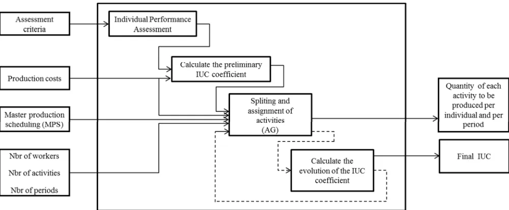
which incorporates competence improvement or depreciation over time. Our modeling approach here is based on a multi-period assignment model which takes into consideration the dynamic evolution of individual competencies. A general assignment problem does not allow highlighting the competence and workload constraints. For this reason, we have characterized each individual by an individual coefficient (IUC) and proposed a mathematical model that allows modeling the dynamic evolution of individual competencies. We have adopted the following logic to model and solve the problem of programming activities that simultaneously consider the three constraints: workforce versatility, equitable distribution of workload and dynamic evolution of competencies. The principal of the resolution method is illustrated as following (Figure 2.2). In this work, we are interested in minimizing the assignment cost while allowing improving individual competencies.

3. MODELING OF OPERATORS’

EFFICIENCIES

Each operator in the manufacturing industry masters one or more activities with consideration to the operators’ efficiencies in different competences. The workforce can be characterized relying on three dimensions: primarily, the ‘’work performance’’ secondly, the ‘’execution quality’’ and finally, the “consumption ratio”. In this work, we adopted the actors’ characterizations discussed by [18]. Therefore, we express an actor’s ability to achieve a given activity via three indicators:

WP WP Q Ts Q_{Tr Q} (1)

EQ EQ Q Qg_Q (2)

CR CR Q CR

Q . _Qcn

(3)

With,

! : The amount of activity (i) assigned to be

1451

Qg : Compliant production of activity (i) produced by operator (j) at period (p);

Ts : standard time required to execute _! ;

Tr : real time spent in executing _!;

" : Number of components required to produce

one unit of the activity (i);

k : index of component;

#$ : Number of the component (k) required to

produce one unit of the activity (i);

% !$ : The amount of component (k) consumed by the operator (j) at the period (p) to produce the activity (i).

Where, WP represents the “work performance” of the operator (j) demonstrated at the period (p) when performing the activity (i);

EQ is the “execution quality” of the operator (j) demonstrated at the period (p) when performing the activity (i)

CR is defined as the ratio between the total production carried out by the individual (i) and the quantity of raw material used by the some individual to obtain this total production.

In the next section, we will formulate the extra cost resulting from the assignment of a given activity (i) to a given operator (j) whose initial performance is not optimal. The demonstration is presented in four steps: the first step concerns the extra cost due to additional time related to the working speed; the second step calculate the extra cost due to non-compliant products, the third step calculate the extra cost due to the loss of components which are improperly handled and the fourth step presents a combination of the three extra costs.

3.1. Calculation of the extra cost due to the additional time

The extra time (Ta) to produce the quantity demanded ( & ≡ () is defined as:

Ta*Qd, Tr*Qd, - Ts*Qd,

*1 - WP,. Tr*Qd, (4)

Let,

Ts*Qd, Ts. Qp Ts.Qd_EQ (5)

Replacing (5) in (1), we get:

Tr*Qd, _{WP ∗ EQ ∗ Qd}Ts (6)

Substituting (6) in (4), the extra time due to the additional time is:

Ta*Qd, _{WP ∗ EQ . Ts. Qd}1 - WP (7)

Assume that the average hourly rate (AHR) corresponds to the overall charges to be covered divided by the number of invoiced hours. The extra cost (Cat) due to the additional time

*Ta,to produce *Qd,is equal to:

Cat*Qd, Ta*Qd, ∗ AHR 1 - WP

WP ∗ EQ . Ts. Qd. AHR

(8)

3.2. Calculation of the extra cost due to poor product:

If (EQ < 1), so how much it is the extra cost due to the “non-compliant products”.

Let,

non-compliant products *1 - EQ,. Qp

*1 - EQ,.45₆₄

(9)

Assume that (Cr) corresponds to the production cost and (Cnq) is the extra cost due to those “non-compliant products” is equal to:

Cnq *Qd, 1 - EQ_{EQ . Qd. Cr} (10)

3.3. Calculation of the extra cost due to the loss of raw material:

If (CR < 1), then there is a damaged components due to improper use. Consequently, how much it is the extra cost ( 8₉, due to those “damaged components”? Assume that (8":_$) corresponds to the purchase cost of components (k), then (8₉) is:

C5 ;*Qc - Qp ,. Cmp

=

Thus,

C5 ; >1 - CR_{CR ? . Qp . Cmp}

=

C5 ; >1 - CR_{CR ? . n . Qp. Cmp}

ISSN: 1992-8645 www.jatit.org E-ISSN: 1817-3195

1452

C5 Qd_{EQ . ; >}1 - CR_{CR ? . n . Cmp}

=

Therefore,

C5 Qd_{EQ . @; >CR . Cmp ?}n

=

- ;*n . Cmp , =

A

(11)

Assume that (8": _{BC D}) corresponds to the raw material cost needed to produce one unit, with:

*8": BC D ∑$$ #$. 8":$,. So, we get:

C5 Qd_{EQ . @; >CR . Cmp ?}n

=

- Cmp FG HA

(12)

We pose the following hypothesis: 8I_$ %JK,

∀ N. So, CR O∏ CR Q CR

Therefore:

C5 Qd_{EQ . @; >CR . Cmp ?}n

=

- Cmp FG HA

Thus:

C5 Qd_{EQ . R}Cmp_CR FG Hé- Cmp FG HT

Finally we get:

C5 1 - CR_{EQ. CR . Qd. Cmp} FG H (13)

3.4. Calculation of the total extra cost:

Considering the expressions of Cat, Cnq and Cd are given previously in (8), (10) and (13), the total extra cost (Ct) due to the individual underperformance is equal to:

Ct*Qd, Cat*Qd, U Cnq*Qd, U 8&* &, (14)

Then,

Ct *Qd,

>1 - WP_{WP. EQ . Ts. AHR U}1 - EQ_{EQ . Cr}

U1 - CR_{EQ. CR . Cmp} FG Hé? . Qd

(15)

Divide this expression by (Qd) gives the extra cost per unit produced (Csu):

Csu 1 - WP_{WP. EQ . Ts. AHR U}1 - EQ_{EQ . Cr}

U1 - CR_{EQ. CR . Cmp} FG Hé

(16)

We considered that the production cost (Cr) is equal to the sum of the raw material cost

( 8": _{BC Dé} ∑$_$ #_$. 8":_$ ) and the

manufacturing cost (AHR*Ts), so:

Cr Cmp FG Hé U AHR. Ts (17)

We set:

α Cmp_Cr FG Hé (18)

Replacing the above expressions given in (17) and (18) in (16), we get:

Csu >_{WP ∗ EQ . *1 - α, U}1 - WP 1 - EQ_EQ

U1 - CR_{EQ. CR . α? . Cr}

(19)

We can deduce that the extra cost is directly related to the individual performance which is the combination of the three indicators (WP, EQ and CR). We choose to call this aggregate indicator “the individual underperformance coefficient (IUC)” denoted by:

IUC _{WP . EQ . *1 - α , U}1 - WP 1 - EQ_EQ

U_{EQ . CR . α}1 - CR

(20)

Consequently, the individual (j) is considered as an expert in the activity (i) when (Z[8 0) and this case is possible when ]^ 1 , EQ 1 and CR 1. This formulation will be introduced in the allocation modeling.

4. MODELING THE EVOLUTION OF INDIVIDUAL PERFORMANCE

1453 dynamic vision of the workers efficiency. In workforce assignment model, the learning curve effect on productivity can be used to differentiate the performance of operators in the same activity. Individuals with a higher competency level can carry out certain tasks better or faster than individuals with a lower competency level. In this section, we will propose a modeling of these learning and forgetting phenomena. Each operator can perform a given activity more efficiently if they carry out the same activity as long as possible. The amount of time required to perform this activity will decrease every time the activity is repeated.

This phenomenon was first described by [17] who reported it as one of the factors that affects the cost of airplanes. In recent years, the learning curves are incorporated into the workforce scheduling model. [8] compared performance of existing well-known learning curves using a large set of empirical data and showed how to select appropriate learning curves based on task characteristics. [14] proposed a precedence graph approach based on learning from multiple sources of information available to generate new feasible assembly line balances in mass production of complex product. Others as [15] developed a workforce scheduling model for assigning tasks to multi-skilled workforce by considering learning of knowledge and requirements of project quality. The proposed model is improved by taking account of the upper bound of employees’ experiences accumulation, and the stable performance of mature employees. Regarding the modeling of learning phenomenon introduced in the literature, the most common representation of experience curves is the exponential function of [17]: _ 8 `a. Where: Y is the production cost at unit X; 8is the first unit production cost and b is the learning curve exponent. Based on the exponential representation, we will present a model that analyzes the extra cost expressed in terms of the individual underperformance coefficient (IUC) of an individual whose efficiency is not optimal. Equation (21) describes the evolution of this additional cost with the number of repetitions of work (X):

Csu *X, Csu *1,. Xc ₍₂₁₎

In this equation, the extra cost is represented by the

8de fg *`, value for an operator whose

underperformance is IUC ij, and who is allocated for an activity (i) defined by a standard time (Ts); for this activity, 8de fg *1, is the extra cost found at the first assignment. The parameter “b” can be expressed as: b Log *ri, j,/log *2, where (ri, j)

expresses the learning rate of the individual (j) in the activity (i). The value of 8de fg *`, is the extra cost found after X repetition of the same work by the same operator without interruption. We can then derive the evolution of the efficiency of an actor from the previous efficiency expressed through the value of (IUC), as shown in equation (23). First of all, let us present the following demonstration:

Let, Csu*X, Csu*1,. Xc

With, Cr. IUC*X0, Cr. IUC_{G H pq}. X_rc

So, IUC *X_r, IUC_{G H pq}. X_rc

Let, X_rc _stu stu *vw,

xyxzx{| with, log Xr

c _logstu *vw,

stu xyxzx{|

So, b. log X_r log IUC *X_r, - log IUC _{G H pq}

Then, log X_r q}~ stu *vw,•q}~ stu _c xyxzx{|

Therefore,

Xr 10Rq}~ stu *v

w,•q}~ stu xyxzx{|

c T (22)

At the repetition X `_rU 1 :

IUC *XrU 1, IUC G H pq. *XrU 1,c (23)

Replacing (22) in (23), we obtain:

IUC *XrU 1,

IUC G H pq. *10Rq}~ stu *v

w,•q}~ stu xyxzx{|

c T_{U 1,}c

Therefore, we can model the increase of efficiency based on the number of allocation periods, and depending on the previous operator’s efficiency

(Z[8 *: - 1,). So, in function of the period

allocation (p), the formula becomes:

IUC*p,p€€

IUC G H pq. *10Rq}~ stu * • ,•q}~ stu

xyxzx{|

c T_{U 1,}c

(24)

ISSN: 1992-8645 www.jatit.org E-ISSN: 1817-3195

1454 is:•‚_ƒ •‚ „…. Where •‚_ƒ is the time for the „D† unit of lost experience of the forgetting curve, x is the amount of output that would have been accumulated if interruption did not occur,

•‚is the equivalent time for the first unit of the forgetting curve, and f is the forgetting slope.

In our method, an interruption occurs when an individual is not assigned to the same activity in the next period. According to this exponentially-decreasing representation used by [3] and similar to the previous demonstration, we can model the depreciation of efficiency based on the number of interruption periods and depending on the previous operator’s efficiency (Z[8 *: - 1,), as shown in equation (25):

IUC*p,GH‡ˆ

IUC G H pq. *10Rq}~ stu * • ,•q}~ stu

xyxzx{|

‰ T_{U 1,}‰

(25)

Where Z[8*:,CDŠ‹ is the individual’s underperformance level after a period of interruption (Y), and (f) is the slope of the forgetting curve which can be calculated as follows:

f -Log *ki, j,/log *2,. Where (ki, j) indicates

the forgetting rate of the individual (j) in the activity (i). This rate may vary from one individual to another and from a competence to another. The learning-forgetting relationship is illustrated in (Figure 3.1).

In this part, we summarized everything that has been discussed previously. Let:

! : The amount of activity (i) assigned to be

done by the operator (j) at the period (p)

with _! ∈ • _•‘,, &_!’ K“dK _! 0;

•‘, : Minimum lot size;

Qd : The quantity demanded of the activity (i) at the period (p);

Z[8 ! Z[8 ! : The individual

underperformance coefficient of the operator (j) demonstrated at the period (p) when performing the activity (i).

Z[8*˜‘‘, !_{* ”•–—,}: The initial underperformance

coefficient at the start of the assignment phase after the interruption phase (Figure 3.1). This expression remains constant during the assignment phase. The index p_{* GH‡ˆ,} informs about the last interruption

period (the period when the assignment has occurred).

Z[8* CDŠ‹, !_*š››,: The initial underperformance

coefficient at the start of the interruption phase after the assignment phase (Figure 3.1). This expression remains constant during the interruption phase. The index p_*p€€, informs about the last assignment period (the period when the interruption has occurred).

Therefore,

if p 0

IUC r _WP1 - WPr

r. EQ r∗ *1 - α , U

1 - EQ r

EQ r

U_EQ1 - CR r

r. CR r. α

if p œ 1 IUC

IUC*p€€,_*xyz•ž,.

Ÿ

¡₁₀¢

q}~ st£_x¤*¥¦§,•q}~ stu_{x¤¥*xyz•ž,}*{¨¨,

c ©

U 1

ª « ¬ c

; if Q œ Qq€,

IUC IUC* GH‡ˆ,_*{¨¨,.

Ÿ

¡₁₀¢

q}~ st£_x¤*¥¦§,•q}~ stu_x¤¥*{¨¨,*xyz•ž,

‰ ©

U 1

ª « ¬ ‰

; else

1455 5. THE MODELING APPROACH

In this model, we will assume that each worker can be characterized by his/her capacity to perform one or more activities. On the other hand, worker’s effectiveness is specific to each individual and is measured for each activity. As we have seen, the level of competence of each operator determines his/her coefficient of underperformance (IUC) to realize a defined load. The duration, quality of execution and consumption ratio for each activity is therefore not predetermined but is a result from previous periods of assignments and /or interruptions.

Each actor has his/her own individual coefficient (IUC), which is variable during the assignment process. We recall that our modeling approach deals with a multi-period assignment problem taking into account the dynamic evolution of individual competencies. We are simultaneously pursuing three different objectives. First is to ensure a balanced distribution of workloads. Second objective is to respect the time constraints governing working time. And third and final objective is to find a compromise between the assignment cost and the evolution of individual competencies.

The problem can be presented as follows: A production planning consists of a set of P periods, a set of N activities and a set of M workers; we consider the actors are multi-skilled. The ability of each individual (j) to practice a given activity (i) is expressed through his efficiency in term of his ( Z[8 ,.

In addition to the individuals’ versatility objective, we consider that the company adopts a strategy of the uniform repartition of the workload : the workloads of its employees should be the same for each period. Thus, we will focus at three different targets: minimize the assignment cost; ensure a balance between the workloads required and the individuals’ availabilities and maximize the individuals’ efficiencies. As a result, the problem consisting in minimizing a multi-objectives function which is a subject to a set of allocation constraints. In order to develop individual experience with lower cost, the amount of work of each activity at each period is considered as a decision variable.

5.1. Problem parameters

We have a problem defined by the following parameters:

! : Decision variable related to the amount of

work (i) assigned to be done by the operator (j) at the period (p), _!∈ • _•‘,, &_!’ ¯° _! 0;

&!: The quantity demanded of the activity (i) at

the period (p);

Z[8 !: Operators’ underperformance when the operator (j) performs the task (i) in period (p);

8° : Production cost of the activity (i);

8±² : Virtual penalty cost related to any workload that would finish outside the weekly working hours;

³´ !: Available working hours per period (p) of the

individual (j), it represents the maximum working hours of any individual;

8: : Theoretical production rate of the activity (i);

•‘, : Minimum lot size;

8•!DµD_Š…… : The effective workload at period (p);

8•!µ·_Š…… ∶ Average effective workload at period

(p);

8• !C9_Š…… ∶ Effective workload of the individual (j)

at period (p);

NB} : Number of workers.

5.2. Objective function

We are interested in minimizing the cost of execution of each activity by targeting a better correspondence between the skill levels acquired by each individual and those required by each activity. The objective function is composed of three terms, as shown in equation (30).

F*Q , F *Q , U F¼*Q , U F½*Q , (26)

The first term (F ) represents the additional cost due to underperformance manifested by operators, with standard production cost (Cr) as shown in equation (27) .

ISSN: 1992-8645 www.jatit.org E-ISSN: 1817-3195

1456 the average workload per period, and it favors the solutions with minimum gap.

The term (F_½) represents the fictive gain of individuals’ efficiencies developments. It is calculated as shown in equation (29) by comparing the individuals’ efficiencies after the assignment horizon with the targeted performance level.

F *Q , ; ; ; Cr . IUC . Q G

= q

(27)

F¼*Q , ; ;¾CT=}¿_‡‰‰- CTG5_‡‰‰¾

= q

(28)

With:

CT=}¿_‡‰‰ uÀ¥zÁz_•ÂÂ

ÃÄÁ¥ , ∀ p ∈ L

CTH}H_‡‰‰ _; Q

Cp Å RI=}¿Å TD=}¿ , ∀ p ∈ L

G

CTG5_‡‰‰ _; Q

Cp Å RI Å TD=}¿ ,

G

∀ j ∈ M ; ∀ p ∈ L

RI : The performance of the individual (j) in

carrying out the activity (i) during the period (p), It is calculated from the values of the two indicators (WP) and (EQ): RI WP Å EQ ;

RI=}¿ : This is the average of the performance of workers executing the activity (i) during period (p),

it is calculated as follows:

RI=}¿ ∑ Ès x¤¥

ÃÄÁ¥ •É•ÊËzxyÌ zÍ• {ÊzxÎxzÏ*x, ,

= _{∀ i ∈}

N ; ∀ p ∈ L ;

TD=}¿∶ Workstation availability rate.

F½*Q , ; ; max *0; IUC ‰ G €Ñ 5pH‡

G =

- IUC Hpˆ~‡H ,

(29)

At the end of the identification of the criteria to optimize, the objective function of the problem can be represented as the sum of the three expressions:

Min ; ; ; Cr . IUC . Q G

= q

U ; ; ¾CT=}¿•ÂÂ_{- CT}G5•ÂÂ_¾

= q

U ; ; max 0, IUC ‰ G €Ñ 5pH‡

G =

- IUC Hpˆ~‡H

(30)

5.3. The model constraints:

Individuals’ allocation constraints: these constraints insure that, for each worker and at each period, the individual workload is always lower than or equal to the available working hours HD :

CTG5_‡‰‰ Ò HD ∀ j ∈ M ; ∀ p ∈ L (31)

Quantitative constraints: these constraints insure that for each activity, the total produced quantity for the current period are always equal to the demanded quantity:

; ; Q G

Qd ∀ p ∈ L =

(32)

These constraints insure that, for each activity, the quantity assigned should be greater than or equal to the minimum lot size:

Q œ Qq€, ∀ i ∈ N (33)

6. GENETIC ALGORITHM

1457 of individuals, which are likely to perform better than those of the previous generation. Individuals from the reproductive phase will be inserted by a replacement method into the new population. From generation to generation, the performance of individuals in the population increases. The process is repeated until a defined stop criterion is met.

6.1. Initial population representation

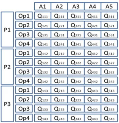
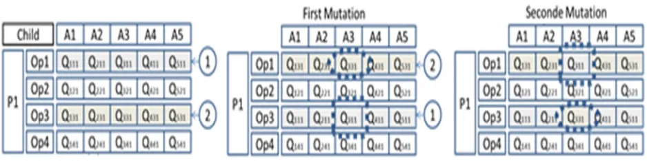
The problem-solving process of genetic algorithms begins with the identification of chromosome representation. In the present article, we describe a genetic algorithm with a matrix form to solve this multi-period assignment problem with multi-skilled workforce. The proposed genetic algorithm is based on a direct encoding of the problem. We will introduce the initial population by generating an initial random chromosome of feasible solutions to form a parent solution, followed by obtaining new solutions and forming new parent through an iterative process. As shown in Figure 5.1, a solution is made up of a matrix form of (n) columns, where (n) is the number of activities and (m) lines, where (m) is the number of workers. This structure is duplicated for each period. Each of the chromosome elements has a value from _•‘, to &_! or _! 0.

Figure 5.1: The solution representation

6.2. Generating an initial population

In this step, an initial population must be generated, where each chromosome represents a solution of the problem. The procedure we used to

generate the initial population of individuals is a guided random generation of (P_size) individuals. This random generation is oriented in such a way that for each activity and for each period, the sum of the quantities allocated to the different operators is equal to the quantity demanded of this activity (Qd ,. For each period (p) and each activity (i), the generation of solutions of the initial population must respect the following constraints:

; ; Q G

Qd , ∀ i ∈ N , ∀ p ∈ L

=

Q œ Qq€, , ∀ i ∈ N

In this phase, each allocation solution does not necessarily respect the capacity constraint. In other words, we accept the violation of capacity constraints when generating the initial population. This capacity constraint will be monitored during the evaluation phase of the objective function.

6.3. Evaluation function

The evaluation phase consists of calculating the fitness of each individual within the population. The main objectives of this work, expressed by the three functions, can be calculated as described above. Despite the genetic algorithms being usually implemented to maximize an objective function [7], our main focus here is to minimize the objective function so that the minimum value will correspond to the best individual. The next step is to determine the fitness of each chromosome. The fitness expression is composed mainly of four terms, as shown in (34). The first three terms represent the basic objective function to minimize. The fourth term allows checking the degree of feasibility of the solutions with respect to the available working hours (HD ). Indeed, the three first terms of the evaluation function are different; we must first normalize each term. The aim of normalization methods is to individually transform each term of the evaluation function to make them homogeneous before combining them. After normalization, the three first terms can be added with an importance weight (Ó_D) associated to each term. As a result, we obtain the following evaluation function:

FéÔpqFpH }G φ FÃ}ˆU φ¼F¼Ã}ˆU φ½F½Ã}ˆU FÖ

(34)

ISSN: 1992-8645 www.jatit.org E-ISSN: 1817-3195

1458

; φH

H ½

H

1 , φHœ 0

FÖ V. CØÙ. ; ; max *0, CTG5_‡‰‰- HD ,

= q

The expression max Ú0, CTG5•ÂÂ- HD Û measures for each period (p) the degree of violation of the available capacity of the actor (j). The factor (V) is a binary variable expressing the capacity constraint violation state: V = 1 for constraint violation and V = 0 for constraint satisfaction.

8±² is a virtual penalty cost related to any

workload that would finish outside the available working hours.

Using this method of normalization and weighting allows us first to favor the possible solutions and to control the compromise between the costs incurred and the development of versatility.

6.4. Selection phase

The selection phase is the determination of individuals from the current population for the reproduction process. The method used is a tournament selection with a tournament size equal to a probability of population size. The selection of a number (k) of individuals is done randomly, then, among this group of individuals, the two best individuals are selected according to the value of their fitness. The other individuals who participated in the tournament are handed over to the population. This procedure is illustrated in Figure 5.2. This method greatly improves the genetic algorithms, because it allows favoring the best chromosomes against the worst ones and ensures no loss among the best individuals found.

6.5. Crossover operator

To obtain new individuals (children) from the selection of two parents, we will use the 1-point crossover operator at the level of the columns of the matrix corresponding to the activities, for each period. This crossing will be carried out as follows (Figure 5.3):

6.6. Mutation operator

Individuals obtained from the crossover phase will undergo the mutation operation. The

mutation operator used is the reciprocal exchange operator. In our approach, this mutation operator is used in two steps. This logic is illustrated in Figure 5.4.

6.7. Insertion operator

Insertion operator is used to improve the overall performance of the population. This insertion allows eliminating the poorest chromosomes from the population. Indeed, individuals that are generated randomly are sorted according to their fitness value in a descending order (in the case of minimization). In our approach, we adopted as type of replacement the Steady-state method.

6.8. Stopping condition

The implementation of genetic algorithms requires the definition of a predetermined stopping. In our approach, we define one stopping criterion, and when it is valid, the exploration will be stopped. The criterion simply depends on the number of generations that were produced. When this maximum number of generations has been run, then the termination procedure occurs. The choice of the maximum number of generations is related to the evolution of the objective function. If the evolution of the fitness no longer seems to evolve, the process is considered to have converged.

7. Illustrative example

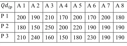
We applied the proposed model on an example of parallel resources which are mainly operators with high added-value. The problem is composed of 8 activities (index A), 4 individuals (index Op), and 4 periods (index P), as shown in tables 7.1 and 7.2.

To describe this problem we need two data sets. The first one, related to the activities to be processed, indicates the theoretical production rates and quantities ordered by period.

Table 7.1: Quantity ordered by period of each activity (in units)

&! A 1 A 2 A 3 A 4 A 5 A 6 A 7 A 8

P 1 _{200 190 210 170 200 170 200 180}

P 2 _{180 150 250 200 220 190 190 190}

1459 P 4 _{170 200 170 220 190 180 170 200}

Table 7.2: Theoretical production rate

A 1 A 2 A 3 A 4 A 5 A 6 A 7 A 8

8: 13 15 18 11 16 18 15 20

The second set of parameters is related to the company: there are different values on the working hours of each individual and the production costs as illustrated by table 7.3. The weekly working hours should not exceed 44 hours.

Table 7.3: The inherent costs of production

A 1

A 2

A 3

A 4

A 5

A 6

A 7

A 8

Cr _{50 51 58 73 63 50 70 69}

8": BC Dé 25 31 31 36 36 33 30 37

α =

8": BC Dé/Cr 0,₅ 0,6₁ 0,5₃ 0,4₉ 0,5₇ 0,6₆ 0,4₃ 0,5₄

We also assume that at the start date of the assignment process, the individual underperformance coefficient (IUC) in the different activities are those shown in table 7.4:

Table 7.4: The initial individual underperformance coefficient (IUC) in the different activities

A 1 A 2 A 3 A 4 A 5 A 6 A 7 A 8

WP

Op1 _{0,76 0,71 0,67 0,9 0,72 0,88 0,76 0,62} Op2 _{0,66 0,65 0,67 0,89 0,86 0,74 0,83 0,87} Op3 _{0,71 0,73 0,7 0,84 0,85 0,61 0,75 0,88} Op4 _{0,81 0,74 0,85 0,82 0,68 0,77 0,83 0,68}

EQ

Op1 _{0,85 0,89 0,93 0,86 0,8 0,85 0,81 0,93} Op2 _{0,94 0,82 0,93 0,8 0,92 0,81 0,8 0,84} Op3 _{0,91 0,95 0,85 0,91 0,85 0,83 0,94 0,9} Op4 _{0,92 0,94 0,91 0,93 0,94 0,85 0,84 0,86}

CR

Op1 0,9 0,92 0,88 0,91 0,9 0,95 0,89 0,92 Op2 0,93 0,9 0,97 0,93 0,91 0,95 0,9 0,9 Op3 0,86 0,89 0,85 0,9 0,9 0,84 0,82 0,87 Op4 0,9 0,92 0,91 0,94 0,92 0,93 0,9 0,88 IUC

Op1 _{0,38 0,31 0,32 0,28 0,48 0,27 0,47 0,31} Op2 _{0,28 0,47 0,26 0,37 0,21 0,39 0,43 0,33}

Op3 _{0,35 0,24 0,45 0,25 0,33 0,52 0,32 0,26} Op4 _{0,25 0,23 0,23 0,21 0,26 0,33 0,36 0,42}

We recall that the closer its value is to 0, the better is the individual competence level. Furthermore, we assume that the learning rate and forgetting rate are the same for all individuals, and which are respectively 80%, corresponding to the parameter (°_, ) and 90% corresponding to the parameter (N_, ). We assume that the (IUC) is calculated for each individual at the beginning of each period based on previous assignments, and it remains constant during the same period. To solve the problem, we must define the company’s preoccupations, namely:

• Case 1: Reduce the losses suffered by the underperformance of the workforce, therefore, use of the most competent individuals. This will not expand the versatility of operators.

• Case 2: Develop the versatility of the actors, the thing that will lead to additional costs,

• Case 3: Seek a compromise between these two extreme cases.

7.1. Case 1: minimization of the extra cost

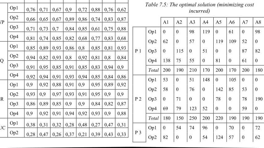
First, we tried to solve the problem with the minimum cost. The assignment solution is summarized in table 7.5, highlighting the amount allocated to each candidate per period for the different activities.

Table 7.5: The optimal solution (minimizing cost incurred)

A1 A2 A3 A4 A5 A6 A7 A8

P 1

Op1 0 0 98 119 0 61 0 98 Op2 62 0 57 0 119 109 52 0 Op3 0 115 0 51 0 0 87 82 Op4 138 75 55 0 81 0 61 0 Total 200 190 210 170 200 170 200 180

P 2

Op1 53 0 51 148 0 105 0 0 Op2 58 0 76 0 142 85 53 0 Op3 0 71 0 0 78 0 78 190 Op4 69 79 123 52 0 0 59 0 Total 180 150 250 200 220 190 190 190 P 3

ISSN: 1992-8645 www.jatit.org E-ISSN: 1817-3195

1460 Op3 58 61 0 0 56 0 134 56 Op4 70 125 86 0 0 103 56 0 Total 210 240 160 150 180 230 190 190

P 4

Op1 0 87 0 121 0 86 0 92 Op2 170 0 67 0 77 0 0 58 Op3 0 0 0 99 113 0 72 50 Op4 0 113 103 0 0 94 98 0 Total 170 200 170 220 190 180 170 200

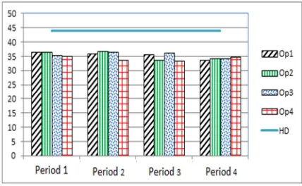
The cost allocation in this case is equal to 64861 (currency unit). Furthermore, the assignment solution respects the constraint of availability of each individual. As shown in figure 7.1, the workload assigned to each candidate is less than its weekly working hours. Thus, the solution respects the uniform load distribution and the operators have more or less the same workload at each period.

Figure 7.1: The workloads distribution of the different actors

However, this solution does not promote versatility. On the other hand, the company loses skills of its operators because of the effect of oblivion. This is shown in the figure 7.3, which shows the evolution of the individual underperformance coefficient (IUC).

7.2. Case 2: minimizing costs associated with individual performance in order to enhance the versatility

In this case, we tried to solve the problem with skill improvement. The assignment solution is summarized in table 7.6, highlighting the amount allocated to each candidate per period for the different activities.

Table 7.6: The optimal solution (skill improvement)

A1 A2 A3 A4 A5 A6 A7 A8

Period1

Op1 0 94 140 0 0 93 81 0 Op2 0 0 0 70 66 77 54 116 Op3 109 0 70 0 134 0 65 0 Op4 91 96 0 100 0 0 0 64 Total 200 190 210 170 200 170 200 180

Period2

Op1 180 65 59 0 0 0 54 0 Op2 0 85 0 92 52 106 0 58 Op3 0 0 129 108 115 0 0 59 Op4 0 0 62 0 53 84 136 73 Total 180 150 250 200 220 190 190 190

Period3

Op1 108 0 52 64 0 96 0 62 Op2 0 58 50 86 106 0 53 0 Op3 102 78 58 0 0 63 85 0 Op4 0 104 0 0 74 71 52 128 Total 210 240 160 150 180 230 190 190

Period4

Op1 57 94 0 0 77 0 113 0 Op2 113 0 0 82 0 71 57 0 Op3 0 0 83 0 113 109 0 145 Op4 0 106 87 138 0 0 0 55 Total 170 200 170 220 190 180 170 200

The cost allocation in this case is equal to 79994 (currency unit). Like in the first case, the assignment solution respects the constraint of availability of each individual. As shown in figure 7.2, the workload assigned to each candidate is less than its weekly working hours. Thus, the solution respects the uniform load distribution and the operators have more or less the same workload at each period.

1461 This solution helps improve versatility. As we can see, the performance of all operators has been indeed improved. This is shown in the figure 7.3, which shows the evolution of the underperformance coefficient.

7.3. Synthesis of the two cases

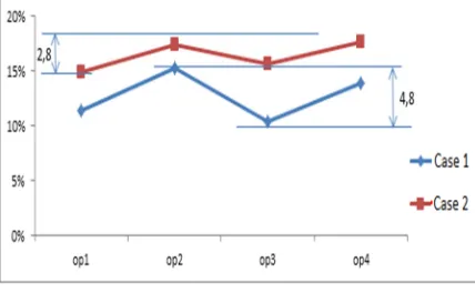
The curves of the figures (Figure 7.3 and Figure 7.4) show the evolution of the average global improvement of the individual underperformance coefficient (IUC) for both cases. For the second case, we observe that the average overall competence rate has improved significantly by (+ 29.13%), as shown in figure 7.3 (change from 12.7% to 16.4%). We can also see that the curve flattened (figure 7.4), this allows to absorb and to minimize the differences between the operators. However, on the other hand we observed an increase in the cost incurred by (+ 23.3%), as shown in Figure 7.5. Improving the level of individual competence has a cost.

Figure 7.3: Evolution of the average global improvement of the individual underperformance coefficient (IUC)

Figure 7.4: Behavior of the change in the individual underperformance coefficient (IUC)

Figure 7.5: Evolution of the cost incurred

Regarding the cost related to the objective of improving competencies by practice, we recall that it is calculated from the difference between the IUC which we hope to get at the end. The IUC values will be obtained at the end of the simulation. The competency goals at the beginning of the simulation are an input data. The solution obtained by the genetic algorithm helps to develop the competency of each individual. This solution, obtained after four periods of simulation, allowed improving the competency of the four operators. However, this development of competency directly causes an increase in the cost incurred by the company.

7.4. Case 3: search of a compromise between reducing the cost incurred and improving individual performance

ISSN: 1992-8645 www.jatit.org E-ISSN: 1817-3195

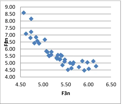
1462 number of objectives to be considered is greater than two. In our case, we will consider two objectives: the first objective is to give information about the cost incurred expressed by (F1), the second is to give information on the evolution of the individual performance expressed by (F3). The other two objectives expressed by the terms (Ü2) and (Ü4) allow to control the distribution of the workload and the constraint of the legal working hours. Figure 7.6 illustrates the density of the points forming the Pareto front.

Figure 7.6: Density of points forming the Pareto front

From figure 7.6, we can see that there is a strong compromise between objective (F1) and objective (F3). The lower the value F1 is, the greater the corresponding F3 value becomes. As we can see, there is not a single solution but a set of solutions that provide the compromise between the two objectives. This compromise is described by the shape of the Pareto front on the basis of which decision-making can be made. The proposed method provides a tool for the multi-period assignment problem in order to minimize the costs incurred and to take into account the operators' skills objectives.

8. CONCLUSION

In this article, we presented a mathematical model and a genetic algorithm approach to solve the workforce multi-periods allocations problem. The scientific difficulty of this problem resides on one hand, in its formulation (problem of multi-period assignment, choice of an indicator of individual competence, choice of a

model of competences evolution and choice of the fitness expression) and on the other hand in its resolution, it is a non-linear problem. The aim of this proposed formulation is to take account of individual competences, their dynamic development and the equitable distribution of the workload. Taking these three factors into account, led us to make changes to the expression of the objective function. For this purpose, we have incorporated an individual performance coefficient (IUC) in the proposed model in which a mathematical expression of (IUC) has been proposed. In addition to the explicit integration of the notion of competence through the use of the coefficient (IUC), two penalty costs were added, the first cost is due to the dissatisfaction of the work distribution constraints and the second cost is related to non-respect of versatility. Considering the both constraints of the equitable distribution of the workload and the versatility in the assignment problem, leads to a rotation in the execution of all activities, which promotes the learning of human resources and developing the flexibility of individuals.

9. REFERENCES

[1] Attia, E.-A., Edi, H.K. and Duquenne, P. Flexible resources allocation techniques: characteristics and modeling, Int. J. Operational Research, 14(2), (2012), pp.221-254.

[2] Bellenguez-Morineau, O. and Néron, E. A Branch-and-Bound method for solving Multi-Skill Project Scheduling Problem, Operations Research, 41(2), (2007), pp.155-170.

[3] Carlson, J. G. and Rowe, R. G. How much does forgetting cost? Indust. Eng. 8(9), 1976, pp.40-47

[4] Drezet, L-E. and Billaut, J-C. A project scheduling problem with labour constraints and time-dependent activities requirements, Int. J. Production Economics, Vol. 112, No. 1, (2008), pp.217–225.

[5] Duquenne, P., Edi, H.K. and Le-Lann, J.-M. Characterization and modelling of flexible resources allocation on industrial activities, In : 7th World Congress of Chemical Engineering. Glasgow, Scotland, (2005).

[6] Edi, K.H. Affectation flexible des ressources dans la planification des activités industrielles: prise en compte de la modulation 4.00

4.50 5.00 5.50 6.00 6.50 7.00 7.50 8.00 8.50 9.00

4.50 5.00 5.50 6.00 6.50

F

1

n

1463 d’horaires et de la polyvalence, PhD Thesis, Université Paul Sabatier, Toulouse, France, (2007).

[7] Goldberg, D.E. Genetic Algorithms in Search, Optimization and Machine Learning, Addison Wesley Longman Publishing Co., Inc, (1989).

[8] Grosse, E. H., Glock, C. H., and Muller, S. Production economics and the learning curve: a meta-analysis, International Journal of Production Economics, vol.170, (2015), pp.401–412.

[9] Gutjahr, W.J., Katzensteiner, S., Reiter, P., Stummer, C. and Denk, M. Competence-driven project portfolio selection, scheduling and staff assignment, Central European Journal of Operations Research, Vol. 16, No. 3, (2008), pp.281–306.

[10] Heimerl, C. and Kolisch, R. Scheduling and staffing multiple projects with a multi-skilled workforce, OR Spectrum, Vol. 32, No. 2, (2009), pp.343–368.

[11] Hlaoittinun, O., Bonjour, E. and Dulmet, M. Managing the competencies of team members in design projects through multi-period task assignment, Collaborative Networks for a Sustainable World: IFIP Advances in Information and Communication Technology, Vol. 336, (2010), pp.338–345.

[12] Hlaoittinun O. Contribution à la construction d’équipes de conception couplant la structuration du projet et le pilotage des compétences. Thèse de doctorat en Automatique, Université Franche-Comté, France, (2009).

[13] Jaber, M.Y. and Bonney, M.C. Production breaks and the learning curve: the forgetting phenomenon. Applied Mathematical Modelling, 20(2), (1996), pp.162-169.

[14] Otto, C. and Otto, A. Multiple-source learning precedence graph concept for the automotive industry, European Journal of Operational Research, vol.234, no.1, (2014), pp.253–265.

[15] Shujin, Q., Shixin, L., and Hanbin, K. Piecewise Linear Model for Multiskilled Workforce Scheduling Problems considering Learning Effect and Project Quality. Hindawi Publishing Corporation. Mathematical Problems in Engineering. Volume 2016, (2016), Article ID 3728934, 11 pages

[16] Valls, V., Perez, A., and Quintanilla, S. Skilled workforce scheduling in Service Centres. E. J. of Operational Research, 193(3), (2009), pp.791-804.

[17] Wright, T. Factors Affecting the Cost of Airplanes. J. of Aeronautical Sciences, 3, (1936), pp.122-128.

ISSN: 1992-8645 www.jatit.org E-ISSN: 1817-3195

1464

Figure 2.1: Illustration of the study context

1465

Figure 3.1: Illustration of the effect of the learning-forgetting curve