Complexity of the gale string problem for equilibrium computation in games

Complexity of the Gale String Problem for

Equilibrium Computation in Games

Marta Maria Casetti

Thesis submitted to the Department of Mathematics London School of Economics and Political Science

for the degree of Master of Philosophy

Declaration

I certify that this thesis I have presented for examination for the MPhil degree of the London School of Economics and Political Science is based on joint work with Julian Merschen and Bernhard von Stengel, published in [4]. The improvement given by Proposition 2.4, and the consequent extensions of Theorem11 and Theorem 12 to the case ofdodd, are an original result.

The copyright of this thesis rests with the author. Quotation from it is permitted, provided that full acknowledgement is made. This thesis may not be reproduced without my prior written consent.

Abstract

This thesis presents a report on original research, extending a result published as joint work with Merschen and von Stengel in Electronic Notes in Discrete Mathematics[4]. We present a polynomial time algorithm for two problems on labeled Gale strings, a combinatorial structure introduced by Gale [11] that can be used in the representation of a particular class of games.

These games were used by Savani and von Stengel [25] as an example of exponential running time for the classical Lemke-Howson algorithm to find a Nash equilibrium of a bimatrix game [16]. It was therefore conjectured that solving these games was a complete problem in the classPPAD(Polynomial Parity Argument, Directed version, see Papadimitriou [24]). In turn, a major motivation for the definition of PPAD was the study of complementary pivoting methods, such as the Lemke-Howson algorithm.

Our result, unexpectedly, sets apart this class of games as a case where a Nash equilibrium can be found in polynomial time. Since Daskalakis, Goldberg and Papaditrimiou [6] and Chen and Deng [5] proved that finding a Nash equilibrium in general normal-form games is PPAD-complete, we have a special class of games, unless PPAD=P.

Our proof exploits two results. As seen in Savani and von Stengel [25] [26], we represent the Nash equilibria of these special games as Gale strings. We then give a graph where the perfect matchings correspond to Nash equilibria via Gale strings, and we exploit Edmonds’ polynomial-time algorithm for a perfect matching in a graph [7]. The proof given in Casetti, Merschen and von Stengel [4] covered only the case of even-dimensional Gale strings; here we extend the result to the general case.

Contents

1 Introduction 9

1.1 Vectors and Polytopes . . . 10 1.2 Normal Form Games and Nash Equilibria . . . 12 1.3 Computational Problems and Complexity . . . 14

2 Labels, Polytopes and Gale Strings 20

2.1 Bimatrix Games and Labels . . . 21 2.2 Cyclic Polytopes and Gale Strings . . . 33 2.3 Gale Games . . . 38

3 Algorithmic and Complexity Results 43

3.1 Polynomial Parity Argument . . . 44 3.2 The Lemke-Howson Algorithm . . . 47 3.3 The Complexity ofAnother Gale . . . 64

4 Further results 73

Acknowledgments 81

List of Figures

2.1 The labeled mixed strategy simplices of a game . . . 23

2.2 The best response polyhedron of a game . . . 24

2.3 The best response polytope of a game . . . 25

2.4 The best response regions of a symmetric game . . . 27

2.5 A degenerate symmetric game. . . 28

2.6 The polytope Pl of a unit vector game . . . 30

2.7 The cyclic polytope C3(6) . . . 33

2.8 A facet of the cyclic polytope C3(6) . . . 36

2.9 A facet of C3(6) as zeroes of the moment curve . . . 36

2.10 The cyclic polytopeC4(6) . . . 37

2.11 A facet ofC4(6) via the moment curve . . . 37

2.12 Not a facet of C4(6) . . . 38

2.13 A labeling ofC4(6) and its completely labeled facets . . . 40

3.1 A PPAD problem . . . 46

3.2 A pivot on the vertices of the cube . . . 48

3.3 A pivot on the facets of the octahedron . . . 48

3.4 A pivot on the vertices of the labeled cube. . . 49

3.5 A pivot on the facets of the labeled octahedron . . . 50

3.6 A Lemke path for a bimatrix game . . . 54

3.7 A game with disjoint Lemke paths . . . 55

3.9 Sign switching of the Lemke Path for Gale Algorithm . . . 61

3.10 Pivoting with sign . . . 62

3.11 The Morris graph forG(6,4) . . . 68

3.12 The graph for a labeling without completely labeled Gale strings 68 3.13 The graph for an labeling withdodd. . . 69

3.14 The second matching of the Morris graph . . . 72

4.1 An Euler complex . . . 75

4.2 The Exchange Algorithm . . . 76

4.3 The endpoints of the Dual Lemke-Howson Algorithm . . . 78

List of Tables

1.1 The prisoners’ dilemma . . . 13

1.2 A coordination game . . . 14

1.3 n-Nash . . . 15

2.1 Another Completely Labeled Vertex . . . 32

2.2 Another Completely Labeled Facet . . . 32

2.3 Gale Nash . . . 39

2.4 Another Gale . . . 41

3.1 End Of The Line. . . 45

3.2 A Lemke path for the Morris labeling . . . 63

3.3 Perfect Matching . . . 64

3.4 Gale . . . 65

List of Algorithms

1 Lemke-Howson . . . 51

2 Dual Lemke-Howson . . . 56

3 Lemke-Howson for Gale . . . 58

4 Completely Labeled Gale String . . . 67

Chapter 1

Introduction

This thesis centers on a problem in the field ofalgorithmic game theory, which concerns the study of strategic interactions from the point of view of computer science. Our result is an algorithm to find a Nash equilibrium in polynomial time for games in a special class, called Gale games.

Gale games can be represented through a combinatorial structure called Gale strings (Gale [11]), using a construction (Savani and von Stengel [25]) on labeled polytopes derived from the game itself (Lemke and Howson [16], Shapley [27]). This connection was used to construct games for which the classic Lemke-Howson Algorithm (Lemke and Howson [16]) takes exponential running time to find a Nash equilibrium (Savani and von Stengel [25]). The Lemke-Howson Algorithm gives a quite straightforward proof of how finding a Nash equilibrium of any two-player game is a problem in the class PPAD (Polynomial Parity Argument, Directed version; Papadimitriou [24]). The PPAD-completeness of the problem has been proven (Daskalakis, Goldberg

indeed a case apart, but because of their tractability, not because of their hardness.

The remainder of this chapter will cover some basic definitions and notation that will be used throughout the thesis, concerning polytopes (see Ziegler [32] for details) in section 1.1, basic game theory (see Myerson [21]) in section 1.2, and computational complexity (see Papadimitriou [23]) in section 1.3.

Chapter2will deal with the geometric and combinatorial constructions leading to the definition of Gale games. In section 2.1 we will see the representation of Nash equilibria of 2-player games as facets or vertices of polytopes built from the game itself. In section 2.2 we will define Gale strings and give the proof of Gale’s theorem, showing the representation of cyclic polytopes as Gale strings. Section 2.3 will then translate the framework of section 2.1 to the point of view of Gale strings, introducing Gale games. In Chapter 3 we will tackle the computational complexity of the issues arising from the previous chapter. After an introduction to the complexity classes related to proofs by parity argument in section 3.1, we will present different versions of the Lemke-Howson algorithm in section 3.2. Finally, in section 3.3, we will present our original result, solving Gale games in polynomial time. A last chapter will relate further results in the field and open problems.

1.1

Vectors and Polytopes

We will often need to refer to sets of natural numbers. We follow the notation [n] ={i∈_N|1≤i≤n}.

An affine combination of points in an Euclidean space zi ∈ Rd, where

i ∈ [m], is P

i∈[m]λizi where λi ∈ R such that P

i∈[m]λi = 1. The points zi areaffinely independentif none of them is an affine combination of the others. Aconvex combinationof the pointsziis such an affine combination withλi ≥0 for all i∈[m]. Theconvex hullof a set Z of points is the set of all its convex combinations. We denote it as conv(Z), so

conv{zi | i∈[m]}={

X

i

λizi | λi≥0 fori∈[m],

X

i

λi= 1}.

A set of points Z is convexif Z = conv(Z). It hasdimension dif it contains exactly d+ 1 affinely independent points. The convex hull ofd+ 1 points of dimension d is called a d-simplex. The standard d-simplexis the convex hull of the first d+ 1 unit vectors, that is, ∆d= conv{ei | i∈[d+ 1]}.

Apolytopeis the convex hull of a finite set of points, not necessarily affinely independent. Its dimension is its dimension as a convex set. Apolyhedron is the intersection of finitely many closed halfspaces {x ∈ _Rd _{| a}>_{x ≤ a0}.} It can be shown that a bounded polyhedron is a polytope. A vertex of a d-dimensional polytope P = conv(Z) is a point z ∈Z that is not the convex combination of other points inP. Anedgeof P is a 1-dimensional line segment that has two vertices as endpoints. A facet of P is a set of dimension d−1 that is the convex hull of a set of vertices that lie on a hyperplane of the form {x ∈ _Rd _{| a}>_{x = a0} so that a}>_{u < a0 for all other vertices u of} P. A d-dimensional polytope P is simplicial if it is the convex hull of a set of at least d+ 1 points v∈ _Rd _{such that nod+ 1 of them are on a common} hyperplane. This is equivalent to requiring that every facet ofP is ad-simplex. A d-dimensional polytope P is simple if every point of P lies on at most d facets. Notice that the points lying on exactlydfacets are exactly the vertices. Consider a polytopeP which has0in its interior and is given byninequalities with normal vectors ci fori∈[n] according to

P ={x∈_Rd _{| c}>

Then the polar of the polytope P is denoted byP∆, where

P∆= conv{ci | i∈[n]}.

If P is a polytope and contains the origin 0, the polar of its polar is P itself, P∆∆ =P. Furthermore, if P is simplicial thenP∆ is simple, and vice versa. For details see Ziegler [32].

1.2

Normal Form Games and Nash Equilibria

The idea ofgameas model of strategic interaction was first introduced by von Neumann [29]. A finite normal form gameis Γ = (P, S, u) where both P and S are finite. Here P is the set of players, and S =×p∈PSp is the set ofpure strategy profiles, whereSp is the set of pure strategiesof playerp. The aim of each playerp∈P is to maximize theirpayoff functionup :S→R. The vector

of payoffs isu=×_p∈Pup. By “game” we will always mean “finite normal form game.” A mixed strategyof playerpis a probability distribution on Sp. It can be described as a point on the (|Sp| −1)-dimensionalmixed strategy simplex

∆p ={x∈_R|Sp| _{| x≥0, 1}>_{x= 1}.}

The set of mixed strategy profiles is the simplicial polytope ∆ = ×_p∈P∆p. We extend the payoff functions to up : ∆ → R linearly. A Nash equilibrium

of a game is a strategy profile in which each player cannot improve their expected payoff by unilaterally changing their strategy; such a strategy is called abest response. Notice that applying a positive affine transformation to all the payoffs does not change the Nash equilibria of the game. The following “best-response condition” is useful and easy to show (e.g., Nash [22]).

The existence of a Nash equilibrium is guaranteed by the fundamental theorem by Nash ([22]). Notice that there can be more than one equilibrium.

Theorem 1. (Nash [22]) Every finite game in normal form has at least one Nash equilibrium.

Bimatrix games are games with only two players. They can be described by two m×n payoff matrices A and B, where aij and bij are the payoffs of respectively player 1 and of player 2 when the former plays her ith pure strategy and the latter plays hisjth pure strategy, andm=|S1|andn=|S2|. A bimatrix game is zero-sum if B = −A, and symmetric if B = A>. We give two classic examples of bimatrix games: the prisoners’ dilemma and the coordination game.

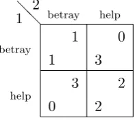
Example 1.1. In the symmetric non zero-sumprisoners’ dilemmaof Table1.1, each player must decide whether to “help” the other one or to “betray” them. If both players help each other, they will get a small reward. If both betray, they will pay a small penalty. If one betrays and the other cooperate the former will get a large reward and the latter will pay a large penalty. The only equilibrium is the profile in which both players betray. If player 2 betrays, the best response of player 1 is to betray, since it gives her payoff 1 instead of 0. If player 2 helps, her payoff for betraying is 3 and her payoff for helping is 2, so betraying is again the best response. The same holds for player 2, so at the equilibrium both players will betray.

@ @ 1 2

betray

help

betray help

1 3

1 0

0 2

3 2

Table1.2 shows a coordination game. Both players can drive on either a mountain or a valley road. They lose if they drive on the same road and win if they avoid each other, regardless of which road they take. The pure strategy Nash equilibria are (mountain, valley) and (valley, mountain). There is also a symmetric equilibrium in mixed strategies which can be represented as the vectors of probabilities ((1/2,1/2),(1/2,1/2)).

@ @ 1

2

mountain

valley

mountain valley

0 1

0 1

1 0

1 0

Table 1.2 A coordination game.

1.3

Computational Problems and Complexity

We base this section on the definitions in Papadimitriou [23], to which we refer for further details.

A deterministic Turing machine M (we will imply the “deterministic” from now on) is a representation of an algorithm that takes an input, runs a algorithm manipulating the input on a tape, and returns an output when it comes to a halting state (if it ever does).

the latter the symbol in the position of the cursor. The transition function returns the next state q∈K, the symbol τ ∈Σ to be written at the position of the cursor, and a direction in which the cursor will move on the tape. The possible directions are “left”, “right”, or “stay”, represented respectively by ←,→,−. The first symbol is never overwritten, and from there the cursor can

only go left.

In some cases, the machine reaches the stateYes(the machineacceptsthe input), No(the machinerejectsthe input) or the halting stateh after a finite amount of time. The output is then given by M(x) =Yes orM(x) =No if the machine accepts or rejects the input. If the halting statehis reached, the output is M(x) = y, where y is the finite (possibly empty) string of symbols that is left on the tape after the symbol Band before any string oft’s at the end. It is also possible that the machine doesn’t halt on input x; we denote this case as M(x) =%.

A problem P that requires an output that is either “Yes” or “No” is a decision problem; its complement is the problem P that outputs “No” for each instance ofP that outputs “Yes”, and vice versa. A problem where the output can be a string M(x) = y on the output tape as above is a function problem; note that no guarantee on the halting state is required. If the output is a string M(x) = y satisfying a relation R(x, y) or the input is rejected if it is not possible to find any such string, the problem is a search problem. A search problem where the input is never rejected is a total function problem. By Theorem 1, the problem n-Nash of Table 1.3is a total function problem.

n-Nash

input : A n-player game.

output: A Nash equilibrium of the game.

Formally, a Turing machine isM= (K,Σ, δ, s), whereK and Σ are finite, Σ∩K = ∅ and Σ always contains the symbols t and B. The transition

functionis δ, defined as follows, where{←,→,−}_*(K∪Σ): δ:K×Σ−→(K∪ {h, Yes, No})×Σ× {←,→,−}.

A slightly different, although equivalent, model allows formultiple strings: k ∈ _N cursors move on k strings σi ∈ Σ∗; the states are still represented as p∈K. The input is given in the tape of the first string; assuming the machine halts, the output is given in the tape of the k-th string.

A language is a set of strings of symbols L ⊆ (Σ\ {t})∗; a class is a set of languages. Let M be a Turing machine, and let x ∈ (Σ\ {t})∗. We say that M decides L if either M(x) = Yes if x ∈ L or M(x) = No if x /∈L. A Turing machine Maccepts L if x∈ L is a necessary and sufficient condition for M(x) = Yes, and if x /∈ L then M(x) = No or M does not halt. Finally, Mcomputesa function f : (Σ\ {t})∗ →Σ∗ ifM(x) =f(x) for every x∈(Σ\ {t})∗.

LetP1 be a problem and let x be an instance of P1 that is encoded in |x| bits. P1 reduces to the problemP2 in polynomial timeif there exists a function f :{0,1}∗ → {0,1}∗, a Turing machineM, and a polynomial p such that for all x∈ {0,1}∗

1. x∈P1 ⇐⇒ f(x)∈P2;

2. Mcomputes f(x);

3. Mstops after p(|x|) steps.

reducible to P2, it takes polynomial time to “translate”P1 toP2, and then to “translate back” a solution ofP2 as a solution ofP1. This is particularly useful ifP2is hard: then the problemP1is at least as “difficult”. Furthermore, if the problem P2 is also complete in a class C, it can be used as a test of belonging to the class C.

The complexity class P (polynomial-time) contains all the polynomially decidable problems, that is, all problems P such that there exists a Turing machine M that outputs either Yes or No for all inputs x ∈ {0,1}∗ of P after p(|x|) steps, wherep is a polynomial. A problemP belongs to the class NP (non-deterministic polynomial-time) if there exists a Turing machineM and polynomials p1, p2 such that

1. for allx∈P there exists acertificatey∈ {0,1}∗ such that|y| ≤p1(|x|);

2. M accepts the combined input xy, stopping after at most p2(|x|+|y|) steps;

3. for all x /∈ P there does not exist y ∈ {0,1}∗ such that Maccepts the combined input xy.

An equivalent definition givesNPas the class of all languagesLfor which the binary relation R(x, y) such thatL ={x | R(x, y) holds for some y} satisfies the following conditions:

1. (polynomially balanced) if (x, y)∈R then|y| ≤ |x|k _{for somek∈}

N;

2. (polynomially decidable) if there is a Turing machine that decides L in polynomial time.

of a problem. Consider for instance theNPproblemHamilton Path, defined as “given an input graph x, is it possible to find a Hamiltonian pathy of x?” There are graphs with more than one possible Hamiltonian path, and each one of these can be used as certificate.

It is quite simple to see thatP⊆NP, but it is an important open problem whether the inclusion is strict. If this were not the case, it could be argued that there isn’t any substantial difference between finding a solution and verifying its validity. This seems to contradict most of the human intellectual experience, where the value of an “original” discovery is perceived as fundamental; the “conventional” view is therefore that P 6= NP. Another open problem is whether NP=co−NP; again, this is widely believed to be false. Notice that if NP6=co−NPthen alsoP(NP, but not vice versa.

The classes FPand FNP are analogous to P and NP, respectively, but for function problems instead of decision problems. Formally,FNP (function non-deterministic polynomial-time) is defined in Megiddo and Papadimitriou [18] as the class of problems of the form “given an x ∈Σ∗, find y ∈ Σ∗ such that (x, y)∈R, where R is a polynomially balanced binary relation, or reject the input.” FP(function polynomial-time) is the class of all FNP problems that can be solved in polynomial time. As in the case of decision problems, it is not known whether FP = FNP; the question is actually equivalent to whether P = NP. Megiddo and Papadimitriou [18] also define the class TFNP (total function non-deterministic polynomial-time) as the class of all FNPproblems where for everyx∈Σ∗a solutiony∈Σ∗is guaranteed to exist. From another point of view, TFNP=F(NP∩co−NP), and the existence of aTFNP-complete problem would imply thatNP=co−NP. The lack of TFNP-complete problems has led to define a number of new classes; we will

see more of this in section 3.1.

problem associated with a binary relationQ(x, y) is “givenx, how many yare there such that (x, y) ∈ Q?” Then #P is the class of all counting problems associated with binary relations that are both polynomially balanced and polynomially decidable. It is interesting to notice that there are #P-complete problems for which the corresponding search problem can be solved in polynomial time. An example close to the topic of this thesis is given in Brightwell [2]: although finding an Eulerian circuit in an undirected graph takes polynomial time, counting the number of possible circuits in the same graph is complete in #P.

Chapter 2

Labels, Polytopes and Gale

Strings

In the remainder of this thesis we focus on bimatrix games. We identify the game with its payoff matrices (A, B), and we assume that both A and B are non-negative, and that neither AnorB> has a zero column; this can be done without loss of generality, by adding a constant to all entries in A and B if necessary.

We start by showing a construction to represent a bimatrix game as two simplices subdivided in labeled regions such that the Nash equilibria of the game correspond to “completely labeled” points of the simplices. This idea is due to Lemke and Howson [16]. As in Balthasar [1] and Savani and von Stengel [26], that together with Savani and von Stengel [25] constitute the main source of material for this chapter as a whole, we follow the very clear approach given by Shapley [27].

be reduced to a problem on the facets or vertices of a labeled polytope, under some simple conditions.

Finally, we further restrict our scope to Gale games, that is, unit vector games for which the polytopes in the previous section can be represented by a combinatorial structure called Gale strings. In the second section of this chapter we define Gale strings and we study how they correspond to a special case of polytopes, called cyclic polytopes, as proven by Gale [11]. The third and last section will combine the results of the previous ones with a definition of labeling for Gale strings; this will lead to a reduction from the problem of finding a Nash equilibrium of a Gale game to the problem of finding a complete labeling for a Gale string.

2.1

Bimatrix Games and Labels

Let (A, B) be bimatrix game, and let X = ∆1 and Y = ∆2 be the mixed strategy simplices of player 1 and 2, respectively, that is,

X = {x∈_Rm _{|x≥0, 1}>_{x= 1},}

Y = {y ∈_Rn _{|y≥0, 1}>_{y= 1}.} (2.1) Alabelingof the setsX andY assigns to eachx∈X andy∈Y a set oflabels, which is a subset of [m+n], as follows:

1. them pure strategies of player 1 are denoted as i∈[m];

2. then pure strategies of player 2 are denoted asm+j withj∈[n];

3. each mixed strategy x∈X of player 1 has

• label ifor each i∈[m] such that xi = 0,

• label m +j for each j ∈ [n] such that the j-th pure strategy of

4. each mixed strategy y∈Y of player 2 has

• label m+j for each j∈[n] such that yj = 0,

• label ifor each i∈[m] such that the i-th pure strategy of player 1 is a best response to y.

This labeling can be used to characterize the Nash equilibria of the game: A pair (x, y) is calledcompletely labeledif each possible label in [m+n] is a label of x or ofy.

Theorem 2. (Shapley [27]) Let (x, y) ∈ X ×Y. Then (x, y) is a Nash equilibrium of the bimatrix game (A, B) if and only if (x, y) is completely labeled.

Proof. The mixed strategyx∈Xhas label m+jfor some j∈[n] if and only if the j-th pure strategy of player 2 is a best response tox. By Proposition 1.1, this is a necessary and sufficient condition for player 2 to play his j-th strategy at every equilibrium where player 1 chooses x. The analogous holds for the strategies y ∈ Y and player 1 playing her i-th strategy in response to player 2 choosing y. Therefore, at an equilibrium (x, y) all labels m+j, with j ∈[n], appear either as labels of x or of y. Conversely, if (x, y) is not completely labeled, then some label does not appear as a label ofxory. This label represents a pure strategy that is played with positive probability but is not a best response, which contradicts the equilibrium property.

Example 2.1. (Savani and von Stengel [26]) Consider the 3×3 game (A, B) with A=     

1 0 0 0 1 0 0 0 1

    

, B =     

0 2 4 3 2 0 0 2 0

     . (2.2)

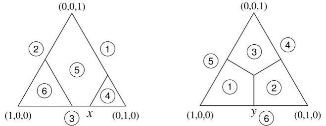
Figure 2.1 shows the mixed strategy simplices X and Y: the exterior facets are labeled with the pure strategy that is played at the opposite vertex of the simplex. The interior is covered by the best response regions, labeled by the other player’s pure best response strategies. For example, the best-response region in Y with label 1 is the set of all the (y1, y2, y3)∈R3 such thaty1 ≥y2 and y1 ≥y3. There is only one pair (x, y) that is completely labeled, namely x= (1₃,2₃,0) with labels 3,4,5, andy= (1₂,1₂,0) with labels 1,2,6. This is the only Nash equilibrium of the game.

6 4 5 2 1 3 (1,0,0) (0,1,0) (0,0,1)

x

y

Figure 2.1 The labeled best response regions of the mixed strategy simplices of player 1 (left) and player 2 (right) in game (2.2).

The representation of a game and its Nash equilibria in terms of best response regions can be translated to an equivalent construction on polytopes. The first step is to notice that the best-response regions can be obtained as projections onX andY of the best-response facets of the polyhedra

P = {(x, v)∈X×_R |B>x≤1v}, Q = {(y, u)∈Y ×_R |Ay ≤1u}.

In P, these facets are the points (x, v)∈X×_Rsuch that (B>x)j =v, which in turn correspond to the strategies x∈X of player 1 that give exactly payoff v to player 2 when he plays strategy j; this payoff is the best-response payoff by the definition ofP. The projection of the facet defined by (B>x)j =vtoX then has labelj. Analogously, the facet ofQgiven by the points (y, u)∈Y×_R such that (Ay)i =u projects to the best-response region of Y with label i.

Example 2.2. (Savani and von Stengel [26]) In Example 2.1, the inequalities B>x≤1v are

3x2 ≤ v 2x1+ 2x2+ 2x3 ≤ v 4x1 ≤ v.

Figure 2.2 shows the best-response facets of P and their projection to X by ignoring the payoff variablev, which gives the subdivision ofXinto best-response regions of Figure 2.1.

(0,0,1) (1,0,0) (0,1,0) v 5 6 1 0 2 3 4 4 3 2 1 0 0 2 3 4 1 4

Figure 2.2 The best response polyhedron of player 1 in game (2.2).

Given the assumptions on non-negativity of A and B>, we can change coordinates to xi/v and yj/u and replace P and Q with the best-response polytopes

P = {x∈_Rm _{| x≥0, B}>_x≤1},

The polytope P is the intersection of the m+n half-spaces that correspond to either player 1 not playing her i-th pure strategy or to a best response j of player 2, where i∈[m] and j∈[n]. The analogous statement holds for Q. Formally, a point x∈P has label kif and only if either xk = 0 for k∈[m] or (B>x)j = 1 for k =m+j with j ∈ [n], and a point in Q has label k if and only if either (Ay)k= 1 for k∈[m] oryj = 0 fork=m+j withj∈[n].

Hence, a point (x, y)∈P×Qis completely labeled if and only if it satisfies thecomplementarity condition that states that for alli∈[m] and allj ∈[n],

xi= 0 or (Ay)i= 1 , yj = 0 or (B>x)j = 1 .

(2.5)

Therefore, if (x, y) ∈ P ×Q is completely labeled either the corresponding point in P×Qis a Nash equilibrium or (x, y) = (0,0); we refer to the latter case as artificial equilibrium.

Example 2.3. (Savani and von Stengel [26]) Keeping on with Example2.1and 2.2, the best response polyhedronP of Figure 2.2becomes the best response polytope of Figure 2.3. Notice that the vertex (x, y) = (0,0) is completely labeled, since it is labeled by the labels 1,2,3 in P and 4,5,6 in Q.

(0,0,0)

1

x x₂

3 x

5

6

4

We now consider some special cases of games and how they are related to each other in terms of computational complexity. First of all, we note that any bimatrix game can be “symmetrized”. This result is due to Gale, Kuhn and Tucker [12] for zero-sum games, while its extension to non-zero-sum games is a folklore result.

Proposition 2.1. Let (A, B) be a bimatrix game and let (x, y) be one of its Nash equilibria. Then (z, z), where z = (xα, yβ) for suitable positive scalars α andβ, is a Nash equilibrium of the symmetric game(C, C>), where

C =  

0 A

B> 0 

. (2.6)

McLennan and Tourky [17] have proven a result in the opposite direction of Proposition 2.1: any symmetric game can be translated into a imitiation game, where the payoff matrix of player 1 is the identity matrixI. In any Nash equilibrium of (I, B), the mixed strategy x of player 1 corresponds exactly to the symmetric equilibrium (x, x) in the symmetric game defined by the payoff matrix of player 2. Since it takes polynomial time in the size of a matrix to calculate its transpose, an algorithm that finds a Nash equilibrium of a bimatrix game can be used to find a symmetric Nash equilibrium of a symmetric game.

Theorem 3. (McLennan and Tourky [17]) The pair (x, x) is a symmetric Nash equilibrium of the symmetric bimatrix game (C, C>) if and only if there is some y such that (x, y) is a Nash equilibrium of the imitation game(I, B) with B =C>.

Example 2.4. (Savani and von Stengel [26]) As an example, consider the symmetric game (C, C>) with

C=     

0 3 0 2 2 2 4 0 0

    

, C>=     

0 2 4 3 2 0 0 2 0

     . (2.7)

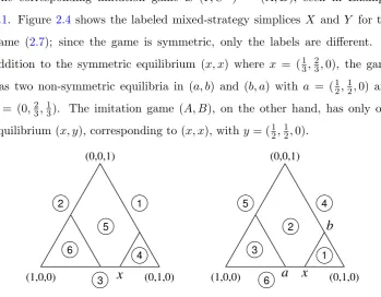
The corresponding imitation game is (I, C>) = (A, B), seen in Example 2.1. Figure 2.4 shows the labeled mixed-strategy simplices X and Y for the game (2.7); since the game is symmetric, only the labels are different. In addition to the symmetric equilibrium (x, x) where x = (1₃,2₃,0), the game has two non-symmetric equilibria in (a, b) and (b, a) with a = (1₂,1₂,0) and b = (0,2₃,1₃). The imitation game (A, B), on the other hand, has only one equilibrium (x, y), corresponding to (x, x), withy= (1₂,1₂,0).

6 4 5 2 1 3 (1,0,0) (0,1,0) (0,0,1)

x

x

b

a

Figure 2.4 The best response regions of the symmetric game (2.7).

strategies against a mixed strategy is never larger than the size of the support of that mixed strategy. Geometrically, this means that no point of the best response polytope P lies on more than m facets and no point of the best response polytope Q lies on more thannfacets, so bothP and Q are simple. Furthermore, a point of P has exactly m labels if and only if it is a vertex, and a point of Qhas exactly nlabels if and only if it is a vertex. Therefore, all completely labeled points (x, y) are vertices of the best response polytopes, and Nash equilibria are isolated points.

Example 2.5. (Savani and von Stengel [26]) An example of degenerate game is given by (C, C>) with

C=     

0 4 0 2 2 2 4 0 0

    

, C>=     

0 2 4 4 2 0 0 2 0

     . (2.8)

As shown in Figure 2.5, the mixed strategy x = (1₂,1₂,0), that also defines the unique symmetric equilibrium (x, x) of the game, has three pure best responses. The Nash equilibria (x, y) of the imitation game (I, C>) are not unique, since any convex combination of (1₂,1₂,0) and (1₃,1₃,1₃) can be chosen fory. 1 3 3 1 2 2 (0,0,1)

(1,0,0)

x

3 1 2 4 5 6 (1,0,0) (0,1,0) (0,0,1)

y

A generalization of imitation games is the class of unit vector games, introduced by Balthasar [1]. These are defined as bimatrix games of the form (U, B) where the columns of the matrix U are unit vectors. By the results above, finding a Nash equilibrium of a bimatrix game is at least as hard as finding a Nash equilibrium of a unit vector game. Savani and von Stengel [26] have shown that the problem of finding a completely labeled vertex of the product of the best response polytopesP×Qcan be simplified for unit vector games: it is enough to find a completely labeled vertex of a single polytope Pl, for which the last nfacets are labeled following a the labeling in [m] that also encodes the matrix U.

Theorem 4. (Savani and von Stengel [26]) Let l : [n] → [m] be a function, and let (U, B) be the unit vector game with U = (e_l(1) · · · e_l(n)).

Let Ni ={j∈[n] | l(j) =i} for i∈[m], and define Pl and Ql as

Pl = {x∈_Rm _{| x≥0, B}>_x≤1},

Ql = {y∈Rn | y≥0, Pj∈Niyj ≤1 for i∈[m]}.

(2.9)

Let lf be the labeling of the facets of Pl with labels in [m]defined as follows:

xi ≥0 has label i for i∈[m], (B>x)j ≤1 has label l(j) for j∈[n].

(2.10)

Then x ∈ Pl is a completely labeled vertex of Pl\ {0} (that is, has all labels in [m]) if and only if there is some y ∈ Ql _{such that, after scaling, the pair} (x, y) is a Nash equilibrium of (U, B).

Conversely, letx∈Pl\ {0}be completely labeled. Ifxi>0, then there is j ∈[n] such that (B>x) =j and l(j) =i; that is,j∈Ni. For all i∈[m] such that xi >0, definey as follows: yj = 1, andyh= 0 for all h∈Ni\ {j}. Then (x, y)∈P ×Qis completely labeled.

Example 2.6. (Savani and von Stengel [26]) The game in Example 2.1 is a unit vector game with l(i) = i. In the polytope Pl of Figure 2.6 the labels 4, 5 and 6 of the best response polytope P of Figure 2.3 are replaced by 1, 2 and 3, since the corresponding columns of A are the unit vectors e1, e2, e3. The only completely labeled point ofPl are the origin0, corresponding to the “artificial” equilibrium, andx, corresponding to the unique Nash equilibrium of the unit vector game (2.2).

x

0

3

1 1

3

2

Figure 2.6 The polytopePl _{of the unit vector game (2.2).}

We now move on the dual version of Theorem 4 given by Balthasar [1]. We can translate the polytope Pl of (2.9) to P ={x−1 |x ∈Pl}, possibly multiplying all payoffs in B by a constant so that 0 is in the interior of P, which holds if 1 in the interior of Pl, that is, all columns bj of the matrix B fulfill 1>bj <1, forj∈[n]. Then

P ={x+1≥0, (x+1)>B ≤1}=

The polar of P is then

P∆= conv({−ei |i∈[m]} ∪ {cj |j∈[n]}) (2.11)

wherecj =bj/(1−1>bj). Since P and P∆ have0in their interior,P∆∆=P. Furthermore, P∆ is simplicial and its facets correspond to the vertices of P and vice versa. We label the vertices ofP∆as the corresponding facets inPl, so the completely labeled facets of P∆ correspond to the completely labeled vertices of Pl. In particular, the facet corresponding to0 is

F0 = {x∈P∆ | −1>x= 1} = conv{−ei |i∈[m]}.

(2.12)

Theorem4 then translates to the following.

Theorem 5. (Balthasar [1]) Let P∆ _{be a labeled m-dimensional simplicial} polytope with 0 in its interior and vertices e1, . . . , em, c1, . . . , cn such that F0 in (2.12) is a facet of P∆.

Let (U, B) be a unit vector game, with U = (el(1) · · · el(n)) for a labeling l: [n]→[m] and B= [b1 · · ·bn], where bj =cj/(1 +1>cj) for j∈[n].

Let lv be the labeling of the vertices of P∆ given by

lv(−ei) = i for i∈[m], lv(cj) = l(j) for j∈[n].

(2.13)

Then a facet F 6=F0 of P∆ with normal vector v is completely labeled if and only if (x, y) is a Nash equilibrium of (U, B), where x= (v+1)/(1>(v+1)), so that xi = 0 if and only if ei ∈ F for i ∈ [m] and the mixed strategy y is the uniform distribution on the set of the pure best replies to x, which in turn correspond to all j∈[n]such that cj is a vertex ofF.

completely labeled facets of P∆ and equilibria of (U, B) with the “artificial” equilibrium corresponding to the facet F0 in (2.12).

Given a bimatrix game (A, B), it takes polynomial time to write and solve the linear equations defining its best response polyhedra P , Q and its best response polytopes P, Q. It also takes polynomial time to label P , Q and P, Q. Analogously, given a unit vector game (U, B), it takes polynomial time to construct and label the polytope Pl and its polar. Therefore, Theorem 4 gives a polynomial time reduction from the problem 2-Nash to the problem

Another Completely Labeled Vertexof Table2.1and Theorem5gives a dual reduction to the problemAnother Completely Labeled Facetof Table2.2.

Another Completely Labeled Vertex

input : Anm-dimensional simple polytopeP withm+nfacets; a labeling lf : [m+n]→[n]; a vertexv0ofP that is completely labeled bylf. output: A vertexv6=v0 of P that is completely labeled by lf.

Table 2.1 The problemAnother Completely Labeled Vertex.

Another Completely Labeled Facet

input : A simplicial m-dimensional polytope P∆ with m+n vertices; a labeling lv : [m+n] → [n]; a facet F0 of P∆ that is completely labeled by lv.

output: A facetF 6=F0 of P∆ that is completely labeled by lv.

Table 2.2 The problemAnother Completely Labeled Facet.

Proposition 2.2. 2-Nashreduces in polynomial time toAnother Completely

2.2

Cyclic Polytopes and Gale Strings

We now apply the results of the previous section to unit vector games for which the best response polytope is the dual of a cyclic polytope. These polytopes are characterized by their representation as a combinatorial structure, called Gale strings. We will first define cyclic polytopes, then Gale string, then we will give the theorem by Gale [11] that shows the equivalence of the two representations.

Themoment curve in dimension dis defined as

µd:R−→Rd µd:t7−→(t, t2, . . . , td)>. (2.14) The cyclic polytope Cd(n) in dimension d with n vertices, where n > d, is given as the convex hull of any n points on the moment curve, that is, by n arbitrary realst1, . . . , tn, wheret1 <· · ·< tn, according to

Cd(n) = conv{µd(ti) | 1≤i≤n}. (2.15)

Example2.7. Figure2.7shows the cyclic polytope in dimension 3 with 6 facets.

Figure 2.7 The cyclic polytopeC3(6).

Given k ∈ N and a set S, we can represent the function f : [k] → S as

1k for a run of length k and 0k for a string of 0’s of length k. AGale string of length n and dimension d, where n > d, is a bitstring s that satisfies the following conditions:

1. exactly dbits ofsare equal to 1;

2. (Gale Evenness Condition) 01k0 is a substring of s ⇒ kis even.

We denote by G(d, n) be the set of Gale strings of lengthnand dimension d. In general, the Gale Evenness Condition allows for Gale strings that start or end with an odd-length run; if dis even thenscan start with an odd run if and only if it ends with an odd run. When dis even, we can therefore see the Gale strings inG(d, n) as “loops” obtained by “gluing together” the endpoints of the strings; on these “loops” all runs are even. Formally, we can see the bit positions in a Gale string s ∈ G(d, n) with d even as equivalence classes modulo n.

Example 2.8. As an example for even d, we have

G(4,6) ={111100,111001,110011,100111,001111,

011110,110110,101101,011011}

The strings111100,111001,110011,100111, 001111and 011110 are equivalent under a cyclic shift (if considering the strings as “loops”, the 1’s are all consecutive), as are the strings 110110, 101101 and 011011 (two runs of two 1’s separated by a single 0). As an example for oddd, we have

G(3,5) ={11100,10110,10011,11001,01101,00111}.

Notice that because dis odd, a cyclic shift is not allowed: 01011is a shift of 10110 but it is not a Gale string.

The relation between cyclic polytopes and Gale strings was given by Gale [11].

Theorem 6. (Gale [11])For any d, n∈_N, where n > d, a set F is a facet of Cd(n) if and only if

Proof. First, a hyperplane in Rd of the form {x ∈ Rd | a>x = a0} for some nonzero vector a = (a1, . . . , ad)> can contain at most d points on the moment curve, because otherwise the polynomial equation with a polynomial of degree dgiven by −a0+a1t+a2t2+· · ·adtd= 0 would have more than d roots t. For the same reason, any dpoints on the moment curve are affinely independent and define a unique hyperplane through them, which the moment curve crosses at these points. Notice that if the curve were tangent to the hyperplane at an intersection, then a slight perturbation of the hyperplane could contain d+ 1 ord−1 points on the moment curve.

Lett1<· · ·< tdbe a choice ofdof thetj’s in the definition (2.15) ofCd(n); then the intersection of the moment curve and of the hyperplane H through the points µd(t1), . . . , µd(td) coincides exactly with the points µd(ti). Since the moment curve crosses the hyperplane at all intersections, ift, t0 ∈ {/ ti}and t < ti < t0 for exactly one of the ti’s then µd(t) and µd(t0) are on opposite sides of H.

A facet F of the cyclic polytope Cd(n) is given by F =H∩Cd(n). This corresponds to a choice of ti’s such that for all the other tk∈ {/ ti | i∈[d]}in the definition of Cd(n), the corresponding µd(tk) are on the same side of H. This can happen only if for every pair of these tk’s the moment curve has an even number of crossings at µ(ti) of H between them. This is equivalent to ask that there is an even number of ti’s between any twotk’s.

Let sbe the bitstring in which the 1’s correspond to theti’s and the 0’s correspond to the other tk’s. Then the condition that the set F in (2.16) is a facet is equivalent to the Gale Evenness Condition.

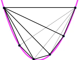
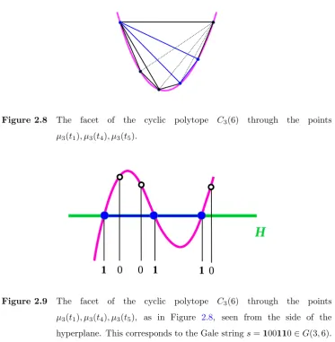
Example 2.9. Consider the facetF of the cyclic polytopeC3(6) marked in blue in Figure2.8. Let us label the vertices on the moment curve asti, withi∈[n], and we set s(i) = 1 if ti is a vertex of F and s(i) = 0 otherwise. Figure 2.9 represents the intersection of the moment curve and the hyperplane H inR3

defined by the ti such that s(i) = 1. This shows how the corresponding Gale string s∈G(3,6) is s=100110.

Figure 2.8 The facet of the cyclic polytope C3(6) through the points

µ3(t1), µ3(t4), µ3(t5).

H

1

0

0

1

1

0

Figure 2.9 The facet of the cyclic polytope C3(6) through the points

Example 2.10. Figure 2.10shows the cyclic polytope C4(6), with the exterior facet corresponding to the Gale string s = 111100. Figure 2.11 shows the correspondence between the string s = 111100 and the intersection of the moment curve and the hyperplaneH.

5 6

1 3

2

4

Figure 2.10 The cyclic polytope C4(6). The thin lines represent the edges inside the exterior facet, in bold lines. Vertexicorresponds to ti.

H

0 0

1 1

1 1

Figure 2.11 The facet of the cyclic polytope C4(6) given by the intersection of the moment curve and the hyperplane H through the points

µ4(t1), µ4(t2), µ4(t3), µ4(t4). This corresponds to the Gale string

Example 2.11. As a counterexample, consider Figure2.12. The points t=t3 and t0 = t5 lie on the moment curve, but µ4(t3) and µ4(t5) are on opposite sides of the hyperplaneHdefined by the other four points. The corresponding bitstring is s=110101, which is not a Gale string. The violation of the Gale Evenness Condition corresponds to the change of side with respect to the hyperplane between tand t0.

H

1

1

1

1 ₀ 0

Figure 2.12 There is a change of side between two µ4(tj)’s (for the 0 bits). The bitstrings=1101011does not satisfy the Gale Evenness Condition, and the set ofµ4(ti)’s (for the1bits) does not define a facet ofC4(6).

2.3

Gale Games

We now apply Theorem 6 to the study of bimatrix games. By Proposition 2.2, solving 2-Nash can be reduced to Another Completely Labeled

Facet; if the polytopeP∆ in Theorem5 is cyclic, we can exploit Theorem 6 to translate this special case of 2-Nashto a problem on Gale strings.

in G(d, n) has exactydbits equal to 1, a Gale string is completely labeled if and only if for each j∈[d] there is exactly one i∈[n] such that s(i) =1 and ls(i) =j.

Notice that, given a labeling ls : [n]→ [d], it may not always be possible to find a Gale strings∈G(d, n) that is completely labeled by ls.

Example 2.12. For ls= 121314, there are no completely labeled Gale strings. The labels ls(i) = 2,3,4 appear only once in ls, so we must have s(2) = s(4) =s(6) = 1. We also must havels(i) = 1 for exactly onei= 1,3,5. The candidate strings are thens1=110101,s2= 011101,s3= 010111, but none of these satisfies the Gale Evenness Condition.

AGale gameis a unit vector game (U, B) whereU = [el(1)· · ·el(d)] for some labeling l : [n]→ [d] and for which the dual of the best response polytope is a cyclic polytope P∆ = conv{e1, . . . , ed, c1, . . . , cn}. We define the problem

Gale Nashas in Table 2.3

Gale Nash

input : A Gale game.

output: A Nash equilibrium of the game.

Table 2.3 The problem_{Gale Nash}.

Theorem5gives the labeling (2.13) for thed+nvertices of P∆ as

lv(−ei) = i fori∈[d], lv(cj) = l(j) forj∈[n].

We define the labelingls: [d+n]→[d] of G(d, n) as

ls(i) = i fori∈[d], ls(d+j) = l(j) forj∈[n].

(2.17)

Example 2.13. Given the string of labelsls= 123432, there are four associated completely labeled Gale strings in G(4,6): sA = 111100, sB = 110110, sC =100111 and sD =101101. These correspond to the completely labeled facets for the labeling shown in Figure2.13 on the left.

A

B

2

C

1 3

4

3

2 D

facet 1 2 3 4 3 2

A 1 1 1 1 0 0 B 1 1 0 1 10 C 10 0 1 1 1

D 10 1 1 0 1 Figure 2.13 The cyclic polytope C4(6), where the labeling of the vertices

corresponds to the labeling ofG(4,6) given byls= 123432.

The completely labeled facetsA,B,C andD correspond respectively to the completely Gale strings sA = 111100, sB = 110110, sC =

100111andsD=101101.

We can now define the problem Another Gale as in Table 2.4. For brevity, we change the notation from d+n ton.

Another Gale

input : A labeling l : [n]→ [d], where d < n. A Gale string s∈G(d, n), completely labeled by l.

output: A Gale string s0 ∈ G(d, n), completely labeled by l, such that s06=s.

Table 2.4 The problem_{Another Gale}.

It takes polynomial time to translate the facets of the cyclic polytope Cd(d+n) into the corresponding Gale strings in G(d, d+n), following the proof of Theorem 6. Defining the labeling ls from the labeling lv also takes polynomial time: for the labelsi∈[d] it is immediate, for the labelsd+j, where j ∈[n], we have to check thed×nmatrixU of the imitation game. Therefore, by Proposition2.2, we have a reduction fromGale NashtoAnother Gale.

Proposition 2.3. The problem Gale Nash of Table 2.3is polynomial-time

reducible to the problem Another Gale of Table 2.4.

Proposition2.3 can be improved: it is enough to consider the case where dis even.

Proposition 2.4. The problem Another Gale of Table2.4 is reducible to

the case where dis even.

Proof. Consider an instance of the problemAnother Galewith dodd. Lets0₀∈G(d+ 1, n+ 1) be the string defined as

s0₀(i) =s0(i) fori∈[n], s0₀(n+ 1) = 1.

holds in all the interior runs ofs0₀. Let nowl0 : [n+ 1]→[d+ 1] be the labeling defined as

l0(i) =l(i) fori∈[n], l0(n+ 1) =d+ 1.

(2.18)

Notice thats0₀ is completely labeled byl0, since for every for eachj∈[d] there is exactly one i∈ [n] such that s0₀(i) = s0(i) = 1 and ls(i) =j, and the only occurrence of the label d+ 1 is at index n+ 1, where s0₀(n+ 1) =1.

Lets0 be any bitstring of lengthn+ 1 such thats0(n+ 1) = 1, and letsbe the bitstring of length n such that s(i) =s0(i) for i∈[n]. First of all, notice that if s0 ∈ G(d+ 1, n+ 1) then s ∈ G(d, n): it is obtained by removing a bit that is equal to 1, and the Gale Evenness Condition still holds in all the interior runs. Furthermore, ifs0 is completely labeled forl0, thens0(n+ 1) = 1, since the only occurrence of label d+ 1 is at indexn+ 1 and for all the other labelsj ∈[d] there is exactly one i∈[n] such thats(i) =1 and ls(i) =j.

Chapter 3

Algorithmic and Complexity

Results

In the previous chapter we have defined some problems of the form “find another completely labeled” vertex, facet or Gale string; in this chapter we finally study the complexity of these problems. A solution of Another

Completely Labeled Vertex is given by the classic algorithm first introduced by Lemke and Howson [16]. In turn, the Lemke-Howson algorithm prompted the definition of the classesPPADandPPAby Papadimitriou [24]; the definition of these classes is given in the first section of this chapter.

The Lemke-Howson algorithm can be used to prove that the “another completely labeled” problems are in the complexity class PPAD. It is interesting to notice that all this proof can be seen as ultimately relying on Shapley’s [27] work discussed in the previous chapter, see Savani and von Stengel [25], Merschen [19], and V´egh and von Stengel [28]. In the second section we relate the different versions of the Lemke-Howson algorithm and the consequent proof that the “another completely labeled” problems are in the class PPA. We first use it to solve Another Completely Labeled

argument. Finally, we focus on Another Gale and give the full proof that it belongs to the PPAD complexity class, following the clear exposition in Merschen [19]. We close the section with an example of a labeling, due to Morris [20], for which the Lemke-Howson-Gale Algorithm has exponential running time. This is the labeling that Savani and von Stengel [25] have used to construct “hard to solve” games.

The third and last section presents our original result: a polynomial time algorithm for Another Gale, that is, a proof that Gale Nash is in FP. UnlessPPAD = P, this goes in the opposite direction of our first conjecture of PPAD-completeness suggested by the “hard to solve” games by Savani and von Stengel [25]. Our proof relies on a theorem by Edmonds [7] that gives a polynomial-time algorithm to find a perfect matching of a graph or decide that it is not possible to find one. The key of the proof is the construction of a graph from any string of labels such that the perfect matchings of the graph correspond to the completely labeled Gale strings for the labels. We first prove theFPcomplexity of finding one of these completely labeled Gale strings, then we extend the proof to find the second string required by Another Gale.

3.1

Polynomial Parity Argument

As mentioned in section1.3, Megiddo and Papadimitriou [18] have proved that, unless NP = co−NP, the class TFNP (total function non-deterministic polynomial-time) does not have complete problems. To circumvent this limitation, Papadimitriou [24] focused on the argument that proves that a problem inTFNPhas indeed a solution. To study this he introduced, among others, the classes PPA (Polynomial Parity Argument) and PPAD (Polynomial Parity Argument, Directed version).

have a solution by a proof employing the argument “in any directed graph in which all vertices have indegree and outdegree at most one and there is asource (a node with indegree zero) there must be asink(a node with outdegree zero).” Formally: a polynomial-sized circuit withn input bits and m output bits is a function C : {0,1}n _{→ {0,1}}m _{that can be represented with polynomially} many standard “logic gates”. We define PPAD as the class of problems reducible to the problem End Of The Line, see Table 3.1. This is the definition given in Daskalakis, Goldberg and Papadimitriou [6]; the original definition in Papadimitriou [24] is given in terms of polynomial-time Turing machines instead of polynomial-sized circuits.

End Of The Line

input : Two polynomial-sized circuits S and P with n input bits and n output bits such that P(0n_{) = 0}n_6=S(0n_).

output: An inputx∈ {0,1}n _{such thatP(S(x))6=x orS(P(x))6=x6= 0}n

Table 3.1 The problem_{End Of The Line}.

cycle

isolated point

path sink

standard source

source S(x)

P(x) x = P(S(x))

x = S(P(x))

Figure 3.1 A PPAD problem as a directed graph with maximal indegree and outdegree 1.

The input is given by the circuitsS (in green) andP (in red) and the standard source (the yellow node). These circuits are used to define paths (in black), cycles (in blue) and isolated points (in purple). The output can be either a sink (a red node) or a nonstandard source (a green node).

The Line graph. We have that PPADS ⊆ PPAD ⊆ PPA; it is an open problem whether the inclusion is strict.

As we have already noticed, the problem n-Nash, see Table 1.3, is a total function problem. Papadimitriou [24] proved that it belongs to TFNP. Daskalakis, Goldberg and Papadimitriou [6] and Chen and Deng [5] have later proven itsPPAD-completeness, the former forn≥3 and the latter forn≥2. A small amendment of the proof in [6] can be found in Casetti [3].

Theorem 7. (Daskalakis, Goldberg and Papadimitriou [6]; Chen and Deng [5])For n≥2, the problem n-Nash isPPAD-complete.

3.2

The Lemke-Howson Algorithm

Theorem 7 suggests that the study of solutions of n-Nash as endpoints of paths can yield interesting results about the complexity of the problem itself. In this section we will study an algorithm that describes exactly this idea.

p

ivot

F’ F

F₁ F₂

x

y

x₂ x₁

Figure 3.2 A pivot from vertexxto vertexy on the edge of a cube.

G

p

ivot

F

v₂

v₁

x

x’

F₂ F₁

Suppose now that there is a labelinglf : [n]→[d] of the facets of the simple polytopeP. If we pivot from vertexxto vertexx0 we “leave behind” a facetF with labelkto whichxbelongs, butx0does not. At the same time, we “reach” a facetF0with labelh, to whichxdoes not belong, butx0does. Therefore, ifx has labels (l1, . . . , k, . . . , ld), then x0 has labels (l1, . . . , h, . . . , ld). We call this dropping label k and picking up label h, orpivoting on label k; see Figure 3.4. Analogously, if there is a labelinglv : [n]→[d] of the vertices of the simplicial poytope P∆ and we pivot from a facet F with labels (l1, . . . , k, . . . , ld) to a facetF0 with labels (l1, . . . , h, . . . , ld), we say that wedrop labelk and pick up label h, or that wepivot on label k; see Figure3.5.

k h

(l₁ ,l₂,h)

l₂ l₁

(l₁ ,l₂,k)

l₂ l₁

k

h (l₁,l₂,h) (l₁,l₂,k)

Figure 3.5 A pivot on label k: drop a facet with labels (l1, l2, k) and pick up a facet with labels (l1, l2, h).

Consider a labeling functionl: [n]→[d], and a subsetSof [n] with|S|=d. Then S is called almost completely labeledif

l(S) = {l(s)|s∈S} = [d]\ {k} (3.1)

that is, all labels appear once in S except for onemissing label k∈[d]. Since |S| = d, in that case there is one duplicate label h ∈ [d] that appears twice

inS.

The algorithm by Lemke and Howson [16] finds one Nash equilibrium of a bimatrix game. In a modern description (e.g., Savani and von Stengel [25]), it employs pivoting on the vertices of a simple polytope, moving through a succession of almost completely labeled vertices with missing label k, where this polytope is the product P × Q of the best-response polytopes. This can be abstracted slightly further by considering only a single polytope P in dimension d with facets labels from [d]. Algorithm 1 gives this latter version; for simplicity of notation, we will call it Lemke-Howson Algorithm. Algorithm1also computes a “Lemke path”, in the terminology of Morris [20]; this, in turn, can be used to prove some fundamental properties of both the Lemke-Howson Algorithm and the Nash equilibria of a bimatrix game.

Algorithm 1:Lemke-Howson

input : A simple d-polytope P withnfacets and a labeling lf : [n]→[d] of the facets of P. A vertex x0 ofP that is completely labeled by lf.

output: A vertexx6=x0 ofP that is completely labeled by lf.

1 choose any labelk∈[d] as missing label

2 pivot on labelkfrom x0 tox reaching a new facet with labelh

3 while h6=k, so x is not completely labeled do

4 pivot away from the other facet with label hfrom x tox0 5 leth be the label of the new facet of x0

6 setx=x0

7 return x

Proposition 3.1. The Lemke-Howson Algorithm 1 returns a solution to the

PPA problem Another Completely Labeled Vertex. Furthermore, the

number of completely labeled vertices in a simple polytope with labeled facets

Proof. We first show that the Lemke-Howson Algorithm works. From the completely labeled vertex x0, there is a unique edge that leaves the facet with label k which leads to a new vertex x, as in step 2 of the algorithm. If x is completely labeled, then the algorithm terminates with output x, and it is trivial to see that x 6= x0. Otherwise, x is an almost completely labeled vertex with duplicate labelh, where one of the facets that containxand have labelhis a “new” facet that did not contain the preceding vertex on the Lemke path. SinceSis simple,xis always on exactlydfacets and the duplicate label is unique. Hence no vertex, including x0, can ever be re-visited on the path because it would otherwise offer an alternative way to proceed when the vertex was encountered for the first time.

The parity result is proven by the following argument: each Lemke path is uniquely determined by its missing label and its starting point, so the Lemke path from the endpoint with the same missing label will lead back to the starting point. Since the endpoint and the starting point are different, the Lemke paths must connect an even number of points.

Finally, for each label k ∈[d] chosen in line 1 of Algorithm 1, the Lemke paths are disjoint paths connecting all the completely labeled vertices of P, with a standard starting point x0. The problem Another Completely

Labeled Vertex corresponds to finding a non-standard endpoint of this graph, which is a PPA problem.

Proposition3.1 can be extended. Lemke paths can be used to prove that

usually normalized, by multiplication with−1 of all signs if necessary, so that the artificial equilibrium has index −1; then a nondegenerate game with n Nash equilibria with index +1 has n−1 Nash equilibria with index −1. For an in-depth study of the topics related to sign in the Lemke-Howson and other algorithms, we refer to V´egh and von Stengel [28].

Applying the parity result of Proposition3.1to the case of a bimatrix game (not necessarily a unit vector game), and remembering that the point (0,0) corresponds to the “artificial” equilibrium, we have the following result, due to Lemke and Howson [16].

Theorem 8. (Lemke-Howson [16]) Every non-degenerate bimatrix game has an odd number of Nash equilibria.

There are two ways of using the Lemke-Howson Algorithm to find a Nash equilibrium of a bimatrix game (A, B). The first one is to “symmetrize” the game as in Proposition 2.1. Let R = {z ∈ Rm+n | z ≥ 0, Cz ≤ 1} be the

polytope associated to the game (C, C>), where

C=

0 A B> ₀

.

The facets ofCcorrespond to 2(m+n) inequalities. We label both thei-th and the (m+n+i)-th inequality as i∈[m+n] and we apply the Lemke-Howson algorithm starting from the vertex 0. This returns a Nash equilibrium (z, z) of C, which corresponds to a Nash equilibrium (x, y) =z of (A, B). We can also follow the “traditional” exposition of the Lemke-Howson Algorithm given by Shapley [27]. In this version, we alternate a move on the best response polytopes P and a move on the best response polytope Q of (2.4). Since the polytopes P and Qare in Rm and Rn, whereasR is a polytope inRm+n, the

Example 3.1. (Savani and von Stengel [26]) Consider the 3×3 game (A, B) of Example2.1. A=     

1 0 0 0 1 0 0 0 1

    

, B =     

0 2 4 3 2 0 0 2 0

     .

The best response polytopes can be represented as the best response regions of Figure 2.1extended to the origin0, as in Figure 3.6.

The path starts from (0,0). We choose the missing label 1 and move in the polytope P. Then label 6 is duplicate; so we drop it and we make the next move on the polytope Q, and so on until we reach the pointx inP and y inQ, which gives here the only Nash equilibrium (x, y) of (A, B).

0 5 4 6 2 1 3 x 0 3 2 1 4 6 y 5

Figure 3.6 Lemke path for missing label 1 on the best response polytopes of player 1 (left) and player 2 (right) of game (2.2).

Example 3.2. (R. Wilson, cited in Shapley [27]) Consider the symmetric game (C, C>) with

C =     

0 3 0 2 2 0 3 0 1

     . (3.2)

There are three equilibria of (C, C>), all of them symmetric, at (xi, xi) with x1= (0,0,1),x2= (1/6,1/3,1/2) and x3 = (1/3,2/3,0).

All Lemke paths from the artificial equilibrium (0,0) end at (x1, x1), and consequently all other Lemke paths connect (x2, x2) and (x3, x3); see Figure 3.7. 0 5 4 6 2 1 3 x₁ x₂ x₃ 0 2 1 3 4 6 y₁ y₂ y₃ 5

Figure 3.7 The Lemke paths for missing label 1 (yellow), 2 (green) and 3 (pink) on the best response polytopes of game (3.2).

The paths for missing label 4, 5 and 6 on the best response polytope of player 1 are the same as the paths of 1, 2 and 3 on the best response polytope of player 2, and vice versa.

The dual version of the Lemke-Howson Algorithm 1 and of Proposition 3.1 is straightforward; analogously, the proof can be extended to show that

Algorithm 2:Dual Lemke-Howson

input : A simplicial m-polytopeP∆ withnvertices and a labeling lv : [n]→[d] of the vertices of P∆. A facetF0 of P∆ that is completely labeled by lv.

output: A facetF 6=F0 of P∆ that is completely labeled by lv.

1 choose any labelk∈[d] as missing label

2 pivot on labelkfrom F0 toF which has a new vertex with label h 3 while h6=k, so F is not completely labeled do

4 pivot away from the other vertex with label h fromF toF0 5 leth be the label of the new vertex of F0

6 setF =F0

7 return F

Proposition 3.2. The Dual Lemke-Howson Algorithm2returns a solution to

the PPADproblemAnother Completely Labeled Facet. Furthermore,

the number of completely labeled facets in a simplicial polytope with labeled

vertices is even.

By Theorem4and Theorem5, in the case of unit vector games it is enough to apply the Lemke-Howson Algorithm 1 to the polytope Pl in (2.9), or the Dual Lemke-Howson Algorithm2to the polytopeP∆in (2.11). The following theorem by Savani and von Stengel [26] guarantees that not only does this yield a Nash equilibrium, but no potential solutions are “lost” considering the polytope Pl with m labels instead of the product of polytopes P ×Q with m+nlabels; an analogous result holds for the dual case.

Theorem 9. Let (U, B) be a unit vector game, with U = [el(1)· · ·el(n)]for a labeling l: [n]→[m]. Let

as in (2.4), and let

Pl={x∈_Rm _{| x≥0, B}>_{x≤1} with labels in [m]as in (2.10)} as in (2.9). Then for the missing label k ∈ [m] the Lemke path on P ×Q projects to a path on P that corresponds to the Lemke path on Pl for the missing label k. For the missing label k = m+j, where j ∈ [n], the Lemke path on P×Q projects to a path onQ that corresponds to the Lemke path on Pl for the missing labell(j).

We finally focus on the case of Gale games. In line with Proposition 2.3, we look for solutions of the problem Another Gale, see Table 2.4. By Proposition2.4, it is enough to study the case of Gale stringss∈G(d, n) with deven. We will consider these as “wrapped-around strings”.

Algorithm 3:Lemke-Howson for Gale

input : A labelingls: [n]→[d], where dis even, such that there is a completely labeled Gale strings0∈G(d, n).

output: A Gale string s∈G(d, n) thats is completely labeled byls, such thats6=s0.

1 choose a missing labelk∈[d]

2 pivot on labelkfrom s0 tosreaching a new 1bit with label h 3 while h6=k, so s is not completely labeled do

4 pivot away from the other1 bit in swith label hfrom stos0 5 leth be the label of the new 1 bit ins0

6 sets=s0

7 return s

The next example illustrates the correspondence between the Dual Lemke-Howson Algorithm and the Lemke-Howson for Gale Algorithm.

Example 3.3. Figure 3.8shows the cyclic polytope C4(6) with the labeling

lv(i) = i fori∈[4], lv(5) = 3,

lv(6) = 2.

This corresponds to the labeling ls = 123432 for G(4,6) given in Example 2.13, for which there are four completely labeled Gale strings: sA =111100, sB=110110,sC =100111and sD =101101. These, in turn, correspond to the facets A, B, C and D of C4(6), that are exactly the completely labeled facets forlv.

A

B

3 3

2

4

2

1

facet 1 2 3 4 3 2 A 1 1 1 1 0 0

B 1 1 0 1 1 0 facet 1 2 3 4 3 2

Figure 3.8 Pivoting on label 3 from sA = 111100 to sB = 110110 in the Lemke-Howson for Gale Algorithm corresponds to the pivoting from facetA (edges in green) to facetB (edges in blue) in the Dual Lemke Path Algorithm.

The indicesi = 1,2,4 correspond to the 2-dimensional intersection of

AandB (edges in pink).

The membership ofAnother Galein the complexity classPPA follows from an argument similar to Proposition3.1. We give here the full proof that it is in PPAD, following the exposition given in Merschen [19].

A permutation of elements of an ordered set S is a sequence without repetition; this gives a rearrangement of the elements of S. A transposition is a permutation of exactly two elements. The sign of a permutation is sign(σ) = (−1)m_{, where m is the number of transpositions needed to get} the natural order σ0 = 1. . . n from σ. It is immediate to see that any two permutations that differ in only one transposition have opposite sign.

The sign of an almost completely labeled Gale string s ∈ G(d, n) with missing labelkand duplicate labelhis defined on two different strings. Leti1 be the index ofh reached by the last pivot (the “new” position of the1) and let i2 be the index of h such that s(i2) = 1 before the last pivot (the “old” position of the 1). Let l1 be the string obtained as l0 substituting k to h at indexi1, and letl2 be the string obtained asl0 substitutingktohat indexi2. Notice that sign(l1) =−sign(l2), since they can be obtained from each other applying the transposition (kh).

Consider now the steps of the Lemke paths in the Lemke Path for Gale Algorithm in the case where sign(s0) = +1; the negative case is analogous, with opposite signs. If the first pivot returns another completely labeled Gale strings, this must have negative sign because it has been obtained “jumping” over an odd number of 1’s. For the same reason, if the pivoting returns an almost completely labeled Gale string, we have that sign(l1) = −1, which implies sign(l2) = +1. The next pivoting step drops the labelhfrom indexi2, so again we change sign. This shows that the Lemke Path for Gale Algorithm results in the sign of the completely and almost completely labeled Gale strings “swinging” as in Table3.9. Notice that all the steps of this construction can be done in polynomial time. Orienting all Lemke paths from positive to negative reduces the problemAnother Gale toEnd Of The Line.

Proposition 3.3. The Lemke-Howson for Gale Algorithm3returns a solution

to thePPADproblemAnother Gale. Furthermore, the number of completely