Constraints on physics beyond the Standard Model and its observable effects

(1)

Constraints on Physics Beyond the Standard

Model and Its Observable Effects

Thesis by

Jennifer Kile

In Partial Fulfillment of the Requirements

for the Degree of

Doctor of Philosophy

California Institute of Technology

Pasadena, California

2007

(2)

c

2007

Jennifer Kile

(3)

For Max and Werner, who were always there, and for Dave, Martin, and Fletch,

(4)

(5)

Acknowledgements

First, I would like to thank Profs. Mark Wise and Michael Ramsey-Musolf for their

extensive guidance, many helpful comments, insight, and support during the last six

years. I would also like to thank the other members of my thesis committee, Profs.

John Schwarz and Robert McKeown, for their willingness to examine this thesis.

Next, I would like to thank Dr. Michael Graesser, who was certainly the brains

and main driving force behind the first project that I worked on here at Caltech,

which here is described in Chapter 4.

I would also like to thank Peng Wang, my officemate and collaborator, who put

up with a huge number of dumb questions from me throughout the last several years,

and to Rebecca Erwin, who endured fewer, but nonetheless equally dumb, questions.

Next, I thank Julian von Wimmersperg for keeping me sane during the production

of this thesis, frequent technical advice, and being willing to critique my writings and

talks at length (and I mean at length). Also, I would like to thank my housemate,

Hareem Maune, for occasionally making sure that I remembered to eat, and Lotty

Ackerman, for the substantial amount of chocolate that she provided.

Also thanks to the other graduate students on the fourth floor of Lauritsen Lab,

who didn’t seem to mind my walking into their offices and talking about completely

random things: Mike Salem, Moira Gresham, Donal O’Connell, Ketan Vyas,

Alejan-dro Jenkins, Paul Cook, and Jie Yang.

I would also like to thank the many people, in addition to those already named

above, who contributed helpful comments about the works described in this thesis.

They include N. Bell, V. Cirigliano, M. Gorshteyn, P. Langacker, B. Nelson, P. Vogel,

(6)

Luty, M. Perelstein, and J. Vinet. Also I would like to thank J. Erler for his helpful

information on using the GAPP code.

And, finally, the works in this thesis were supported by U.S. Department of

En-ergy contracts FG02-05ER41361, ER40701, FG02-05ER41361,

DE-FG03-ER40701, and DE-FG-0392-DE-FG03-ER40701, as well as National Science Foundation awards

(7)

Abstract

In this work, we describe three analyses, all of which involve physics beyond the

Standard Model. The first two discussed here are closely related; they use

effec-tive operator analyses to constrain the contributions of physics beyond the SM to

observable processes. The third project involves the investigations of a particular

extra-dimensions model which addresses the cosmological constant problem.

The first project which we will discuss uses the scale of neutrino mass to place

model-independent constraints on the coefficients of the chirality-changing terms in

the muon decay Lagrangian. We list all of the dimension-six effective operators which

contribute to muon decay and Dirac mass for the neutrino. We then calculate the

one-loop contributions that each of these operators makes to neutrino mass. Taking

a generic element of the neutrino mass matrix to be of order_∼1 eV, we derive limits

on the contributions of these operators to the muon Michel parameters which are

approximately four orders of magnitude more stringent than the current experimental

results, and well below near-future experimental sensitivity. We also find two

chirality-changing operators, which, due to their flavor structure, are unconstrained by neutrino

mass yet contribute to muon decay. However, as these two operators differ from

those constrained by neutrino mass only by their flavor indices, we naively expect

their contributions to also be small; if their effects instead turn out to be observable,

this may be an indication of beyond-the-Standard-Model physics with an interesting

flavor structure.

In the second analysis, we again perform an effective operator analysis, this time

applied to Higgs production at a linear collider. Here we include all

(8)

include operators that contain right-handed Dirac neutrinos. We obtain limits on

these operators from electroweak precision observables, the scale of neutrino mass,

and limits on neutrino magnetic moments, and use these limits to constrain the

contributions of these operators to the Higgs production cross-section. Although

we find that all operators containing right-handed neutrinos contribute negligibly to

Higgs production, we do find three operators containing only SM fields which could

have observable contributions at an e+_e− _{linear collider.}

Lastly, we discuss the characteristics of a particular extra-dimensions model

orig-inally proposed by Carroll and Guica [54]. This model has two extra dimensions

compactified into a sphere, a bulk magnetic field, and a bulk cosmological constant.

In this model, the cosmological constant seen by a four-dimensional observer can

be set to zero by fine-tuning the bulk magnetic field against the bulk cosmological

constant. If branes with a tension are added at each of the poles of the two-sphere,

solutions with zero four-dimensional cosmological constant are still possible, but the

compactified dimensions must acquire a deficit angle which depends on the brane

tension. However, the brane tension does not affect the fine-tuning relationship

between the bulk cosmological constant and the bulk magnetic field. This feature

led to the hope that, after this fine-tuning, the model might self-tune, keeping the

four-dimensional cosmological constant zero regardless of what happens to the brane

tension by adjusting the deficit angle. We speculated that this self-tuning property

would imply a massless scalar mode in the perturbed Einstein’s equations; as there

exist very stringent limits on scalar-tensor theories of gravity, a massless scalar mode

would make this model incompatible with observation. We conducted a search for

such modes, and found none which satisfied the boundary conditions. This finding

(9)

List of Figures

1.1 The current experimental status ofν oscillation parameters, taken from [1]. . . 3

1.2 χ2 _{plotted as a function of}_M

H, taken from [42]. The yellow band shows

the region excluded by the direct searches at 95% CL. . . 8

2.1 Contributions from the operators (a)_O_{V , AD}(6)_˜ and (b)_O_{W, AD}(6) (denoted by the shaded box) to the amplitude for µ-decay. Solid, dashed, and wavy lines denote fermions, Higgs scalars, and gauge bosons, respectively.

After SSB, the neutral Higgs field is replaced by its vev, yielding a

four-fermion µ-decay amplitude. . . 23 2.2 One-loop graphs for the matching contributions of the n= 6 operators

(denoted by the shaded box) to then= 4 mass operator_O(4)_{M, AD}. Solid, dashed, and wavy lines denote fermions, Higgs scalars, and gauge bosons,

respectively. Panels (a, b, c) illustrate contributions from _O(6)_B,W, _O(6)_V_˜ , and _O(6)_F , respectively, to _O(4)_{M, AD}. . . 24 2.3 One-loop graphs for the mixing amongn= 6 operators. Notation is as in

previous figures. Various types of mixing (a–g) and self-renormalization

(h–j) are as discussed in the text. . . 30

2.4 Two-loop graphs for the mixing of the n= 6 operators. Only represen-tive graphs for the mixing of the four-fermion operators _O(6)_{F, ABCD} into

(12)

3.2 Contribution of Class A operators (a) _O`

M, AB and (b) OM, ABν to Higgs production . . . 49

3.3 Contribution of Class B operators to Higgs production . . . 52

3.4 Contribution of Class C operators to Higgs production . . . 53

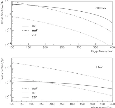
3.5 Ratio of contribution of_OV R,ee to SM Higgs production cross-section for

(top) √s = 500 GeV and (bottom) 1 TeV for CV R,eev2/Λ2 = 10−2. For

√

s= 1 TeV, the line for the Hqq¯,Hµ+_µ₋_{, and}_Hτ+_τ− _{channels is not}

shown; it has the value of ₋2.2, independent of Higgs mass. . . 56 3.6 Ratio of contribution of _OV R,µµ to SM Higgs production cross-section

for (top) √s = 500 GeV and (bottom) 1 TeV for CV R,µµv2/Λ2 = 10−2. Curves for _OV R,τ τ are identical. . . 57

3.7 Ratio of contribution of_OV L,eeto SM Higgs production cross-section for

(top)√s= 500 GeV and (bottom)√s= 1 TeV forCV L,eev2/Λ2 = 10−2. For√s = 1 TeV, the line for theHqq¯,Hµ+_µ₋_{, and}_Hτ+_τ− _{channels is}

not shown; it has the value of 2.6, independent of Higgs mass. . . 59 3.8 Ratio of contribution of _OV Lτ,ee to SM Higgs production cross-section

for (top) √s = 500 GeV and (bottom) 1 TeV for CV Lτ,eev2/Λ2 = 10−2. For√s = 1 TeV, the line for theHqq¯,Hµ+_µ₋_{, and}_Hτ+_τ− _{channels is}

not shown; it has the value of 2.6, independent of Higgs mass. . . 61 3.9 Contributions of operators containing νR to Higgs missing energy final

(13)

Chapter 1

Introduction

The Standard Model (SM) has demonstrated remarkable success in explaining particle

interactions at energies up to a few hundred GeV. The experimental value for the

anomalous magnetic moment of the muon agrees with the SM prediction to seven

significant figures [1]. Fits to the LEP and SLDZ pole data [2] show that the current experimental data is well-described by the the Minimal Standard Model. And, of

course, no non-SM particles have yet been discovered.

However, despite this success, few physicists believe that the SM is valid up to

arbitrarily high energies; the SM contains 19 free parameters (not including neutrino

masses and mixing angles!) which currently must be put in by hand, does not explain

why fermions seem to come in three flavors or predict their masses, and requires the

existence of a Higgs boson with a mass not too far from the weak scale, even though

radiative corrections would be expected to push its mass up to the Planck scale.

Additionally, as the SM does not address the issue of neutrino mass at all, does

not explain the matter-antimatter asymmetry in the universe, and fails miserably to

explain the cosmological constant, we now have conclusive evidence of physics beyond

the SM.

To address some of these issues which the SM leaves unresolved, many ideas

have been proposed for physics beyond the SM. These include supersymmetry (for an

introductory review, see [3]), models of extra dimensions (see reviews [4, 5, 6]), models

with with extra gauge bosons [7], technicolor [8], and many other ideas. Currently, the

(14)

and the cosmological constant problem is a subject of intense study. (For some very

recent reviews on the cosmological constant, see [13, 14, 15].)

While the value of studying particular new physics scenarios is evident, the

rich-ness of possibilities for physics beyond the Standard Model indicates that

model-independent analyses are also worthwhile. In this work, we will use both approaches.

First, in Chapters 2 and 3 we will use general operator analyses to obtain

model-independent constraints on the contributions of new physics to two processes—muon

decay and Higgs production. (Interestingly, both of these processes can, in

prin-ciple, receive contributions from new physics which also gives rise to the

(not-yet-understood) phenomenon of neutrino mass.) Then, in Chapter 4, we will study a

particular extra-dimensions model which attempts to address the cosmological

con-stant problem. We discuss the motivation for each of these analyses below.

1.1

Neutrino Mass and Muon Decay

Although the first direct evidence for neutrino mass came in the 1960s [16] with the

observation of an unexpectedly low νe flux coming from the sun, it wasn’t until the last two decades that the case for nonzero ν mass became compelling. For recent reviews, see [1], [17], and [18]. Fig. 1.1 (taken from [1]) gives a visual summary of

the current knowledge of neutrino oscillation parameters taken from experiments.

Two mass regions in Fig. 1.1 are of particular interest. These roughly correspond

to the regions explored by the “solar” (oscillations ofνe or ¯νeintoν’s of other flavors) and “atmospheric” (oscillations ofνµ) experiments. The former is dominated by the most recent results of Super-Kamiokande (Super-K) [19] and the Sudbury Neutrino

Observatory (SNO) [20], which look for disappearance of solar νe, and KamLAND [21], a reactor experiment which looks for disappearance of ¯νe. Combining the results of the three experiments [19] gives the region marked “Super-K+SNO+KamLAND

95%” in Fig. 1.1, which indicates ∆m2 _{close to 8}_×₁₀−5_eV2 _{and the Large Mixing}

Angle solution for tan2_θ

. Observations of neutral-currentν interactions by SNO [22]

(15)

ν

_µ

↔ν

_τ

ν

_e

↔ν

_X

10

0

10

–3

∆

m

2

[eV

2

]

10

–12

10

–9

10

–6

10

2

10

0

10

–2

10

–4

tan

2

θ

CHOOZ Bugey CHORUS NOMAD CHORUS KARMEN2 PaloV erde

ν

_e

↔ν

τ

NOMAD

ν

_e

↔ν

_µ

CDHSW NOMAD BNL E776 K2K http://hitoshi.berkeley.edu/neutrino Cl 95% Ga 95%

KamLAND

95%

SNO

95%

Super-K

95%

Super-K+SNO +KamLAND 95%

LSND

90

/

99

%

SuperK

90

/

99

%

[image:15.612.116.461.36.592.2]

All limits are at 90%CL unless otherwise noted

(16)

Tha atmospheric neutrino data, however, are dominated by Super-K. They report

in [23] a deficit ofνµ events dependent upon zenith angle and energy, with no corre-sponding deficit in νe events. They thus report sin22θatm > 0.92 and 1.5×10−3 < ∆m2 _< ₃_.₄_×₁₀−3_eV2 _{at 90% CL. They also report [24] a dependence upon} _L/E

(where L is the ν flight distance and E is its energy) in their muon disappearance results, which yields similar results. Finally, they see [25] aντ appearance at the 2.4σ level and find that their results are completely compatible with full νµ−ντ mixing.

Also shown in Fig. 1.1 is the region favored by the LSND experiment [26, 27, 28,

29], whose results favored ¯νµ to ¯νe oscillations with ∆m2 ∼ 1 eV2. Assuming three neutrino flavors, neutrino mass results must satisfy the simple relation

∆m2₁₂+ ∆m2₂₃ = ∆m2₁₃ (1.1)

where ∆m2

ij =m2i−m2j. This relation cannot be satisfied by the ∆m2ijs implied by the solar, atmospheric, and LSND experiments. Thus, the LSND results were considered

possible evidence for a sterile neutrino νs. However, the very recent results of Mini-BooNE [30] do not support the LSND results and there is currently no compelling

evidence for a sterile ν.

While constraints from neutrino oscillations give us information about the squared

mass differences ∆m2

ij between different mass eigenstates, they tell us nothing about

the overall scale of neutrino mass. Results from tritium β decay [31, 32] give a limit of <2 eV [1] on the sum

X

i

|Uei|2m2νi (1.2)

where U is the neutrino mixing matrix.

Limits also exist on the sum of the neutrino masses from cosmology. Constraints

from WMAP and the Sloan Digital Sky Survey [33] give a limit of

X

mν < .42 eV at 95%, CL (1.3)

(17)

It is these last two results which will be the most relevant to our work in Chapters 2

and 3. However, the presence of neutrino oscillations (and therefore nonzero neutrino

mass) imply that the SM Lagrangian is not complete. If neutrinos are purely Dirac

particles, the Lagrangian will receive terms of the form

δ_L =₋mij_νν¯RiνLj +h.c. (1.4)

where i and j are flavor indices. Thus, we must necessarily add a right-handed neutrino νR to the SM. However, if neutrinos are instead purely Majorana particles and receive a mass term of the form

δ_L =₋1 2m

ij

νν¯RiνRcj+h.c. (1.5)

then we find that nature allows lepton number violation. Therefore, when considering

extensions to the SM, we should allow the Lagrangian to contain terms which contain

right-handed Dirac neutrinos or to contain terms which violate lepton number, or

both. In this work, for simplicity, we will assume that neutrinos are purely Dirac

particles.

Given that neutrino mass is a window onto physics beyond the SM, it makes

sense to consider the possibility that the current knowledge of neutrino mass could

already be used to place constraints on new physics and its possible manifestations

in observable processes. The first such process which we consider is muon decay. One

can write the effective muon decay Lagrangian in the form

Lµ−decay ₌

−4√Gµ

2 X

γ, , µ

g_µγ ¯eΓγνν¯Γγµµ (1.6)

where Γγ _{runs over all possible Lorentz structures (1,} _γµ _and _σµν_/√_{2) and} _and

µ are the electron and muon chiralities. In the SM, gV

LL = 1 and all others are

zero. It is easy to see from Eq. 1.6, however, that the sum also includes terms that

(18)

terms which contain right-handed neutrinos, such as the case γ = V, or µ = R. Thus, it is not hard to imagine that if neutrino mass compels us to include in the

Lagrangian effective operators which contain right-handed neutrinos, that some of

these operators could contribute to _Lµ−decay_{. A key point of the analysis which we}

present in Chapter 2 is that some of these operators will contribute to neutrino mass,

and, thus, can be constrained by current limits on mν. (More specifically, one can note that dimension-six operators that contribute to mν without insertions of tiny neutrino Yukawa couplings will contain a single νR field. This implies that the terms in _Lµ−decay _{which can be constrained by limits on} _m

ν will contain one right-handed

ν and one left-handedν, and, thus, ₆=µ.) These coefficients gγ

µ can be translated into effects on the muon decay spectrum,

which can be written as

d2_Γ

dx dcosθ = mµ 4π2W

4

eµG2µ q

x2₋_x2 0

×[FIS(x)±Pµcosθ FAS(x)] (1.7)

×h1 +~ζ_·P~e(x, θ)i

where Weµ = (m2µ+m2e)/2mµ is the maximum e energy, x=Ee/Weµ, x0 =me/Weµ, andP~µandP~eare theµandepolarizations. ~ζis a vector dependent on the experimen-tal configuration. The isotropic and anisotropic components of the decay spectrum,

FIS(x) and FAS(x), can be written in terms of four of the Michel parameters (MPs)

ρ, η, ξ, and δ [34, 35]:

FIS = x(1−x) + 2 9ρ(4x

2

−3x₋x2₀) +ηx0(1₋x) (1.8)

FAS = 1 3ξ

q

x2₋_x2 0

1₋x+ 2 3δ

4x₋3 + q

1₋x2 0−1

. (1.9)

In the SM these parameters take the values ρ=δ = 3₄, η= 0, and ξ= 1.

(19)

gγ µs as

ρ= 3 4 −

3 4 gLRV

2+3

2 gLRT

2+ 3

4Re g S LRgLRT∗

+ (L_↔R)

. (1.10)

It should be noted that the gS,V,T_LR,RL all correspond to terms in Eq. 1.6 which contain right-handed neutrinos. Recently, ρ (and δ) has been measured by the TWIST Col-laboration [36, 37], who hope to eventually improve their precision to the few_×10−4

level.

In Chapter 2, we set out investigate whether the scale of neutrino mass can be

used to place limits on some of the gγ

µ. We enumerate the dimension-six operators

which can contribute to a Dirac mass of the neutrino or to muon decay, and then use

current upper bounds on neutrino mass to derive constraints on contributions of these

operators to chirality-changing (i.e, ₆=µ) terms in the muon decay Lagrangian. We obtain model-independent constraints considerably stronger than the current

experi-mental bounds and, finally, discuss the implications for currently ongoing experiments

to measure the muon decay parameters. The content of Chapter 2 is largely borrowed

from the work of Erwin et al. [38].

In the analysis of Chapter 2 (and later in Chapter 3), we will assume a scale of 1 eV

for an upper limit on a generic entry of the neutrino mass matrix, and, for simplicity,

we will assume that neutrinos are purely Dirac particles. For a similar study of muon

decay where neutrinos are allowed to have Majorana mass terms, see [39]. It should

be noted that our limits from neutrino mass on the effects of physics beyond the SM

given in those chapters will improve if the upper bounds on the neutrino mass scale

become more stringent in future measurements.

One can also ask what ramifications our results can have for certain models. A

class of models for which the Michel parameters have particular relevance is

Left-Right-Symmetric Models (LRSM). For a treatment of the interplay of muon decay

(20)

1.2

Fermionic Operators and Higgs Production

Continuing with our work with effective operators, we move from muon decay to Higgs

production at ane+_e−_{Linear Collider. Unlike muon decay, all that is known about the}

properties of the Higgs boson is theoretical or through indirect experimental evidence.

Direct searches [41] have ruled out the ranges of the Higgs boson massmH <114.4 at the 95% confidence level. Fits to mH by the LEP Electroweak Working Group have yielded the range shown in Fig. 1.2 (from [42]); they obtain a 95% CL upper limit of

186 GeV, which rises to 219 GeV when the direct search results are included.

0

1

2

3

4

5

6

100

30

300

m

_H

[

GeV

]

∆χ

2

Excluded

∆α_had =

∆α(5)

0.02758±0.00035

0.02749±0.00012

incl. low Q2 data

[image:20.612.119.392.240.515.2]

Theory uncertainty

Figure 1.2: χ2 _{plotted as a function of} _M

H, taken from [42]. The yellow band shows the region excluded by the direct searches at 95% CL.

Given the range ofmH compatible with the SM, it (or something like it) is expected to be discovered at the LHC. Assuming that such a Higgslike particle is, in fact,

discovered, a linear collider will be necessary to measure its properties to determine

(21)

particle’s mass, spin, and couplings to other particles. (For a short review, see [43].)

Is the new particle a scalar? Are its couplings to the W± _and_Z _{particles compatible}

with it being the source of electroweak symmetry breaking? Are its couplings to

fermions proportional to their masses? For an excellent discussion of Higgs physics

at a future LC, we direct the reader to [44].

Here, we will concentrate on the observable most relevant to our work in Chapter

3, the Higgs Boson production cross-section. As the production cross-section is also

important for measurements of the Higgs branching fractions [45], we will discuss

their relevance as well.

A precise measurement of the Higgs production cross-section is critical for

distin-guishing an SM Higgs boson from scalars predicted by other models, such as

super-symmetry. For example, the production cross-section for the lightest MSSM Higgs

will differ from that of the SM Higgs. (For a calculation of the cross-sections for

the MSSM Higgses with radiative corrections included, see [46].) In addition, [47]

describes in detail how partial width and branching ratio measurements at a linear

collider could be used to distinguish an SM Higgs boson from an MSSM Higgs. This

would be particularly important for values of tanβ and MA where it is possible that only one of the MSSM scalars would be observable at the LHC.

The branching fractions of a Higgslike scalar can also be useful in

distinguish-ing the SM from extra-dimensions scenarios. The authors of [48] find that an SM

Higgs boson can be distinguished from the Randall-Sundrum scalar radion by precise

measurements of its branching fractions, particularly to gg; for a particularly light radion,ggcan actually be the primary decay mode, whereas a Higgs of the same mass would decay primarily to b¯b. The authors of [49] and [50] consider how Higgs-radion mixing could affect the properties of a Higgs boson; they find that the branching

ratios, particularlyH _→gg, could differ substantially from the SM expectation. [50] additionally find that the HZZ coupling would differ from the SM scenario, leading to changes in the overall Higgs production cross-section.

There are multiple reasons why it is important to understand how much physics

(22)

First and foremost, if it turns out that the possible effects of new physics are large

enough to substantially change either the expected Higgs mass range or its production

or decay mechanisms, search strategies may have to be changed accordingly. Secondly,

given the importance of determining the Higgs production cross-section, we would like

to know whether an observed deviation from the SM expectation favors particular

models, or if unknown new physics at energy scale Λ could make the interpretation

of such a deviation ambiguous.

In Chapter 3, we describe the use of a general operator analysis to constrain the

effects of physics beyond the SM on Higgs production at a linear collider. We restrict

ourselves to dimension-six operators which contain fermions and Higgs fields (for

similar analyses considering other operators, see [51, 52]), including three operators

which we borrow from the muon decay analysis. We then use precision electroweak

data and limits on neutrino mass to place limits on the contributions of these operators

to Higgs production at a linear collider, and find operators that could have observable

effects on the Higgs production cross-section. Chapter 3 borrows heavily from the

work of Kile and Ramsey-Musolf [53].

1.3

Extra Dimensions and the Cosmological

Con-stant

After the discussion of these two model-independent analyses, in Chapter 4 we

inves-tigate the characteristics of a specific model of extra dimensions which was originally

proposed in [54]. This model was proposed to possibly shed new light on the

cosmo-logical constant problem, the observation of a cosmocosmo-logical constant more than 120

orders of magnitude smaller than the naive SM expectation ofM4

P.

Other models of extra dimensions have been proposed to address the cosmological

constant problem [55, 56, 57, 58, 59]. In models with extra dimensions, the

cosmolog-ical constant seen by a four-dimensional observer can receive contributions from both

(23)

models introduce an unpleasant fine-tuning between different terms which contribute

to the cosmological constant. The model presented in [54] also required such a

fine-tuning; however, it appeared possible in this model that, once this fine-tuning took

place, the volume of the extra dimensions would adjust itself so that the cosmological

constant would remain zero, independent of the brane tension.

We expected that this self-tuning property would imply a massless mode in the

perturbed Einstein’s equations, and searched for such modes. The presence of such

a mode would cause this model to be strongly disfavored, as tests of the equivalence

principle [60, 61] place tight constraints on scalar-tensor theories of gravity. We found

no such modes and speculated that this model did not, in fact, have a self-tuning

(24)

Chapter 2

Muon Decay Parameters From

Neutrino Mass

In this chapter, we discuss the first of our two model-independent analyses: using

current limits on the scale of neutrino mass (_∼1 eV) to constrain the effects of new

physics on muon decay. We specifically consider operators which can contribute to

the chirality-changing terms in the muon decay Lagrangian, and we only consider the

case of Dirac neutrinos. The contents of this chapter are, aside from small cosmetic

changes, taken from [38].

2.1

Introduction

Precision studies of muon decay continue to play an important role in testing the

Standard Model (SM) and searching for physics beyond it. In the gauge sector of

the SM, the Fermi constant Gµ that characterizes the strength of the low-energy, four-lepton µ-decay operator is determined from the µ lifetime and gives one of the three most precisely known inputs into the theory. Analyses of the spectral shape,

angular distribution, and polarization of the decay electrons (or positrons) probe for

contributions from operators that deviate from the (V ₋A)_⊗(V ₋A) structure of the SM decay operator. In the absence of time-reversal (T) violating interactions, there

exist seven independent parameters—the so-called Michel parameters [34, 35, 63]—

(25)

anisotropic distribution; and three additional quantities (ξ0_, _ξ00_, _η00_{) that are needed}

to describe the lepton’s transverse and longitudinal polarization1_{. Two additional}

parameters (α0_/A_, _β0_/A_{) characterize a T-odd correlation between the final state}

lepton spin and momenta with the muon polarization: ˆSe·kˆe×Sˆµ.

Recently, new experimental efforts have been devoted to more precise

determi-nations of these parameters. The TWIST Collaboration has measured ρ and δ at TRIUMF [36, 37], improving the uncertainty over previously reported values by

fac-tors of_∼2.5 and_∼3, respectively. An experiment to measure the transverse positron polarization has been carried out at the Paul Scherrer Institute (PSI), leading to

sim-ilar improvements in sensitivity over the results of earlier measurements [64]. A new

determination ofPµξwith a similar degree of improved precision is expected from the TWIST Collaboration, and one anticipates additional reductions in the uncertainties

in ρand δ [65].

At present, there exists no evidence for deviations from SM predictions for the

Michel parameters (MPs). It is interesting, nevertheless, to ask what constraints

these new measurements can provide on possible contributions from physics beyond

the SM. It has been conventional to characterize these contributions in terms of a set

of ten four-fermion operators

Lµ−decay ₌

−4√Gµ

2 X

γ, , µ

g_µγ ¯eΓγνν¯Γγµµ (2.1)

where the sum runs over Dirac matrices Γγ = 1 (S), γα (V), and σαβ/√2 (T), and the subscripts µand denote the chirality (R, L) of the muon and final state lepton, respectively2_{. In the SM, one has} _gV

LL = 1 and all other gµγ = 0. A recent, global analysis by Gagliardi, Tribble, and Williams [67] give the present experimental bounds

on the gγ

µ that include the impact of the latest TRIUMF and PSI measurements.

Theoretically, thegγ

µcan be generated in different scenarios for physics beyond the

1_{The parameters}_η _and _η00 _{are alternately written in terms of the independent parameters}_α/A

andβ/A.

2_{The normalization of the tensor terms corresponds to the convention adopted in [66]. We do}

(26)

SM. The most commonly cited illustration is the minimal left-right symmetric model

that gives rise to non-zerogV

RR,gRLV , andgVLR. From a model-independent standpoint, the authors of [68] recently observed that the operators in Eq. (2.1), having different

chiralities for the muon and final state charged lepton, will also contribute to the

neutrino mass matrix mAB

ν through radiative corrections. Consequently, one expects

that the present upper bounds on mν should imply bounds on the magnitudes of the

gγ

µ. The authors of [68] argued that the most stringent limits arise from two-loop

contributions because the one-loop contributions are suppressed by three powers of

the tiny, charged lepton Yukawa couplings. The two-loop constraints are nonetheless

stronger than the present bounds given in [67] and could become even more so with

the advent of future terrestrial and cosmological probes of the neutrino mass scale.

In this chapter, we present the results of a follow-up analysis of mν constraints on the µ-decay parameters, motivated by the observations of [68] and the new exper-imental developments in the field. Our study follows the approach of [69],[70], and

[71], used recently in deriving model-independent naturalness bounds on neutrino

magnetic moments implied by the scale of mν. We concentrate on the case of Dirac neutrinos, deferring a detailed consideration of Majorana neutrinos to a separate

anal-ysis. Although there exists a long-standing theoretical prejudice favoring the see-saw

mechanism with light, Majorana neutrinos as an explanation of the small scale ofmν, we see several reasons for studying the Dirac and Majorana cases separately:

(i) From the standpoint of string phenomenology, obtaining models with neutrino

self-couplings and a type I see-saw mechanism appears to be quite difficult.

Re-cently, the authors of [72] performed a systematic study of 175 viable ways of

embedding the Standard Model gauge group in theE8_×E8 heterotic string with

Z3 orbifold compactification and found that only two of the twenty classes of such inequivalent models admitted neutrino self-couplings. The natural scale of

mν in these two classes lies many orders of magnitude below the scale implied by neutrino oscillation data. Interactions leading to Dirac masses occur more

(27)

Z3_×Z3 orbifold string construction [73] indicated the plausibility of obtaining a type II see-saw mechanism, wherein left-handed lepton-number-violating

neu-trino self-couplings arise from interactions with scalar SU(2)L triplet fields.

Ei-ther way, however, the appearance of Majorana mass terms is not at all a generic

feature of string constructions, leaving the Dirac case as a logical possibility.

(ii) Experimentally, there exists no conclusive evidence for or against the presence of

light Majorana neutrinos. New searches for neutrinoless doubleβ-decay (0νββ) could provide conclusive proof that the light neutrinos are Majorana, provided

the neutrino mass spectrum has the “inverted” rather than “normal”

hierar-chy (for recent reviews, see, e.g., [74] and [75]). If, on the other hand, future

long-baseline oscillation experiments establish the existence of the inverted

hi-erarchy and/or ordinaryβ-decay measurements indicate a mass consistent with the inverted hierarchy, a null result from the 0νββ searches would imply that neutrinos are Dirac particles3_{. Either way, the investment of substantial}

ex-perimental resources in these difficult measurements indicates that determining

the charge conjugation properties of the neutrino is both a central question for

neutrino physics as well as one that is not settled. Until it is, considering the

implications of Dirac neutrinos remains a valid enterprise.

(iii) The phenomenological analyses of Dirac and Majorana masses for other

neu-trino properties and interactions are quite distinct. As illustrated by the recent

analyses of neutrino magnetic moments in [69], [70], and [71], the characteristics

of the operator basis and renormalization can be sufficiently different and

com-plex for the two cases that separate studies of each are warranted. Moreover, the

parameterization of the µ-decay Michel spectrum in the presence of Majorana neutrinos may require modification from the standard form, as indicated by the

recent work of [76]. Rather than lose the reader in the details of differences in

both the Michel parameterization and operator renormalization for Dirac and

Majorana neutrinos, we prefer to concentrate on the Dirac case in the present

(28)

study and consider the Majorana case in a separate paper.

Having this focus in mind, we work with an effective theory that is valid below a

scale Λ lying above the weak scale v _≈ 246 GeV and that contains SU(2)L_×U(1)Y -invariant operators built from Standard Model fields plus right-handed (RH) Dirac

neutrinos. We consider all relevant operators up to dimension n = 6 that could be generated by physics above the scale Λ. For simplicity, we restrict our attention

to two generations of lepton doublets and RH neutrinos. Extending the analysis to

include a third generation increases the number of relevant operators but does not

change the substantive conclusions. While the spirit of our work is similar to that of

[68], the specifics of our analysis and conclusions differ in several respects:

i) The effective theory that we adopt allows us to compute contributions to mν from scales lying between the weak scale v and the scale of new physics Λ. In contrast, the authors of [68] used a Fierz transformed version of_Lµ−decay _{in Eq.}

(2.1), which is not invariant under the SM gauge group and, therefore, should

be used to analyze only contributions below the weak scale.

ii) We show that for the two-flavor case the operators in _Lµ−decay _{proportional to} g_LRS,T and gS,T_RL arise from twelve independent dimension n = 6 gauge-invariant four-fermion operators, while those containing gV

LR and gRLV are generated by four independent n = 6 operators that contain two fermions and two Higgs scalars.

iii) While the operators that contribute toµ-decay have dimensionn = 6 or higher, the lowest dimension neutrino mass operator occurs at n = 4. The authors of [68] used dimensional regularization (DR) to estimate the mixing between the

n = 6 µ-decay and neutrino mass operators4 _{but did not consider matching}

with the n = 4 operator at the scale Λ that cannot be determined with DR. We derive order-of-magnitude expectations for the n = 6 operator coefficients 4_{Since the computation of [68] did not employ gauge invariant operators, we consider the results}

(29)

implied by this matching, which depends only linearly on the lepton Yukawa

couplings and which gives the dominant constraints for Λv.

iv) For Λ not too different from v, constraints associated with mixing among the

n = 6 operators can, in principle, be comparable to expectations arising from contributions to the n = 4 mass operator. We carry out a complete, one-loop analysis of this mixing and show that only the neutrino magnetic moment and

two-fermion/two-Higgs operators mix with the n = 6 neutrino mass operator to linear order in the lepton Yukawa couplings. We derive the resulting bounds

on the gV

LR,RL that follow from this mixing and find that they are comparable

to expectations based on one-loop matching with the n = 4 mass operator for Λ_∼> v.

v) From the mixing with then= 6 mass operator, we find that the bounds on the

|gV

LR,RL| are two or more orders of magnitude stronger than those obtained in [68] and at least three orders of magnitude below the experimental limits given

in [67].

vi) The neutrino mass implications for the couplingsg_LR,RLS,T are more subtle. Of the twelve independent four-fermion operators that contribute to these couplings,

only eight are directly constrained by the scale of neutrino mass and naturalness

considerations. Based on one-loop matching, we expect that their contributions

to the g_LR,RLS,T are generally _∼104 _{times smaller than the present experimental}

bounds, and_∼103 _{times smaller than obtained in the analysis of [68]. We show,}

however, that the flavor structure of the remaining four operators allows them

to evade constraints implied by either one-loop matching or two-loop mixing.

While from a theoretical perspective one might not expect their contributions to

be substantially larger than those from the constrained operators, experimental

efforts to determine the g_LR,RLS,T remain a worthwhile endeavor.

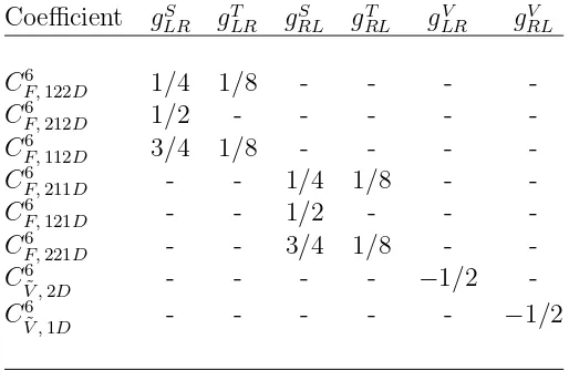
A summary of our results is given in Table 2.1. In the remainder of the paper

(30)

[image:30.612.107.520.186.403.2]

Table 2.1: Constraints onµ-decay couplingsgγ

µ. The first eight rows give naturalness expectations in units of (v/Λ)2_×₍_m

ν/1 eV) on contributions fromn = 6 muon decay operators (defined in Section 3.3 below) based on one-loop matching with the n= 4 neutrino mass operators. For Λ _∼ v, the bounds on gV

LR,RL obtained from one-loop mixing are similar to those listed. The ninth row gives upper bounds derived from a recent global analysis of [67], while the last row gives estimated bounds from [68] derived from two-loop mixing of n = 6 muon decay and mass operators. A “-” indicates that the operator does not contribute to the given gγ

µ, while “None” indicates that the operator gives a contribution unconstrained by neutrino mass. The subscript D runs over the two generations of RH Dirac neutrinos.

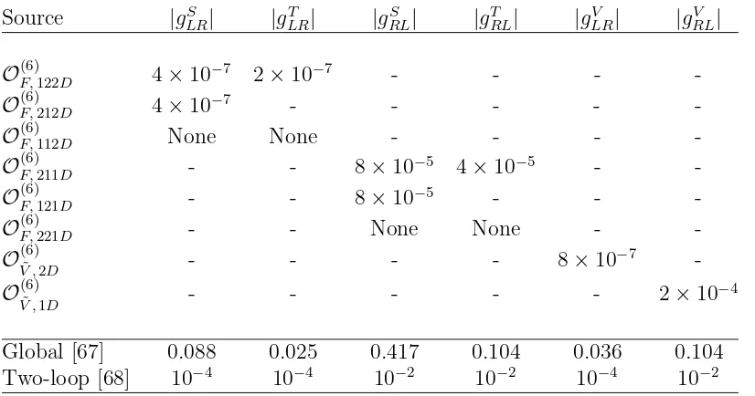
Source _|gS_LR_| _|g_LRT _| _|g_RLS _| _|g_RLT _| _|g_LRV _| _|g_RLV _|

OF,(6)122D 4×10−7 2×10−7 - - -

-OF,(6)212D 4×10−7 - - - -

-OF,(6)112D None None - - -

-OF,(6)211D - - 8×10−5 4×10−5 -

-OF,(6)121D - - 8×10−5 - -

-OF,(6)221D - - None None -

-O_{V ,}(6)˜ ₂_D - - - - 8×10−7

-O_{V ,}(6)˜ ₁_D - - - 2×10−4

Global [67] 0.088 0.025 0.417 0.104 0.036 0.104

Two-loop [68] 10−4 ₁₀−4 ₁₀−2 ₁₀−2 ₁₀−4 ₁₀−2

of independent operators through n = 6 that contribute to mAB

ν and/or µ-decay. Section 2.3 gives our analysis of operator mixing and matching considerations, while

in Section 2.4 we discuss the resulting constraints on theg_LR,RLγ that follow from this analysis and the present upper bounds on the neutrino mass scale. We summarize in

Section 3.6.

2.2

Operator Basis

To set notation, we follow [69] and consider the effective Lagrangian

Leff =

X

n,j

Cn j(µ) Λn−4 O

(n)

(31)

where µ is the renormalization scale, n _≥ 4 is the operator dimension, and j is an index running over all independent operators of a given dimension. The lowest

dimension neutrino mass operator is

O(4)M, AD = ¯LAφν˜ RD (2.3)

where LA _{is the left-handed (LH) lepton doublet for generation} _A_, _νD

R is a RH

neu-trino for generation D, and ˜φ = iτ2φ∗_{, with} _φ _{being the Higgs doublet field. After}

spontaneous symmetry breaking, one has

φ_→



 0

v/√2 

 (2.4)

so that

C_{M, AD}4 _O(4)_{M, AD} _{→ −}mAD_ν ν¯_LAν_RD

mAD_ν = ₋C_{M, AD}4 v/√2 . (2.5)

The other n = 4 operators are those of the SM and we do not write them down explicitly here.

For the case of Dirac neutrinos that we consider here, there exist no

gauge-invariant n = 5 operators. In considering those with dimension six, it is useful to group them according to the number of fermion, Higgs, and gauge boson fields

that enter:

(32)

¯

LγµLLγ¯ µL ¯

`Rγµ`R`¯Rγµ`R ¯

`Rγµ`Rν¯RγµνR ¯

νRγµνRν¯RγµνR ¯

L`R`¯RL ¯

LνRν¯RL

ijL¯i`RL¯jνR

Here `R is the right-handed charged lepton field. Several of the operators appearing in this list can contribute to µ-decay, but only the last one can also contribute to

mAD

ν through radiative corrections. Including flavor indices, we refer to this operator

as

OF, ABCD(6) =ijL¯Ai `CRL¯Bj νRD (2.6) where the indices i, j refer to the weak isospin components of the LH doublet fields and 12 =₋21 = 1.

Fermion-Higgs:

i( ¯LAγµLB)(φ+Dµφ)

i( ¯LAγµτaLB)(φ+τaDµφ)

i(¯`A_Rγµ`_RB)(φ+Dµφ) (2.7)

i(¯ν_RAγµν_RB)(φ+Dµφ)

i(¯`A_Rγµν_RB)(φ+Dµφe)

(33)

mAD

ν since they contain no RH neutrino fields. Any loop graph through which they

radiatively induce mAD

ν would have to contain operators that contain both LH and

RH fields, such as _O_{M, AB}(4) or other n = 6 operators. In either case, the resulting constraints on the operator coefficients will be weak. For similar reasons, the third

and fourth operators cannot contribute substantially because they contain an even

number of neutrino fields having the same chirality and since the neutrino mass

operator contains one LH and one RH neutrino field. Only the last operator

O_{V , AD}(6)˜ ≡i(¯`ARγµνRD)(φ+Dµφe) (2.8)

can contribute signficantly to mν since it contains a single RH neutrino. It also contributes to the µ-decay amplitude after SSB via the graph of Fig. 2.1a since the covariant derivative Dµ contains charged W-boson fields. We also write down the

n= 6 neutrino mass operators

OM, AD(6) = ( ¯LAφνe RD)(φ+φ) (2.9)

as well as the charged lepton mass operator ( ¯Lφ`R)(φ+_φ_{) that we do not use in the}

present analysis.

Fermion-Higgs-Gauge:

¯

LτaγµDνLW_µνa

¯

LγµDνLBµν ¯

`RγµDν`RBµν ¯

νRγµDννRBµν (2.10)

g2( ¯Lσµντaφ)`RWµνa

g1( ¯Lσµνφ)`RBµν

g2( ¯Lσµντaφe)νRWµνa

(34)

As for the fermion-Higgs operators, the operators in (2.10) that contain an even

number of νR fields will not contribute significantly to mABν , so only the last two in the list are relevant:

O(6)B, AD = g1( ¯LAσµνφe)νRDBµν (2.11)

OW, AD(6) = g2( ¯LAσµντaφe)νRDWµνa (2.12)

In addition to these operators, there exist additional n= 6 operators that contain two derivatives. However, as discussed in [69], they can either be related to _O_{B, AD}(6) and _O(6)_{W, AD} through the equations of motion or contain derivatives acting on the νR fields so that they do not contribute to the neutrino mass operator. Consequently,

we need not consider them here. We also observe that the operator _O(6)_{W, AD} will also contribute to the µ-decay amplitude via graphs as in Fig. 2.1b. We have com-puted its contributions to the Michel parameters and find that they are suppressed

by _∼(mµ/Λ)2 _∼<1.7×10−7 relative to the effects of the other n= 6 operators. This suppression arises from the presence of the derivative acting on the gauge field and the

absence of an interference between the corresponding amplitude and that of the SM.

Finally, we note that the operators whose chiral structure suppresses their

contribu-tions to the neutrino mass operator (as discussed above) may, in general, contribute

to muon decay via the terms in Eq. (2.1) having = µ. We do not consider these terms in this study.

2.3

Operator Renormalization: Mixing and

Match-ing Considerations

In analyzing the renormalization of operators that contribute to both µ-decay and

mAD

ν it is useful to consider separately two cases: (i) one-loop matching conditions

(35)

W φ

νD

R

lR

φ

W φ

νD

R

L

(a) (b)

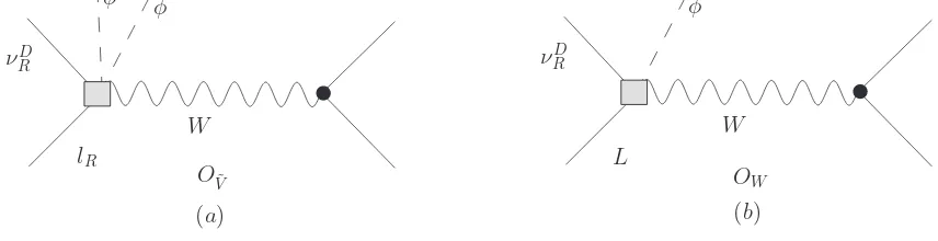
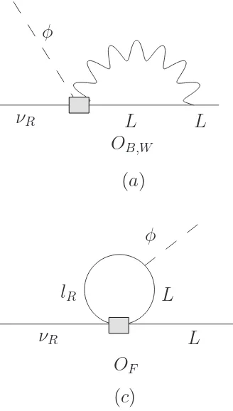
[image:35.612.111.539.34.144.2]

O_V˜ OW

Figure 2.1: Contributions from the operators (a) _O(6)_{V , AD}_˜ and (b) _O_{W, AD}(6) (denoted by the shaded box) to the amplitude for µ-decay. Solid, dashed, and wavy lines denote fermions, Higgs scalars, and gauge bosons, respectively. After SSB, the neutral Higgs field is replaced by its vev, yielding a four-fermionµ-decay amplitude.

contributions to mAD

ν involving the second case will be smaller than those implied

by matching with _O(4)_{M, AD} by _∼ (v/Λ)2_{, since} _O(6)

M, AD contains an additional factor

of (φ†_φ₎_/_Λ2_{. We first consider this case and employ dimensional analysis to derive}

neutrino mass naturalness expectations for the n= 6 operator coefficients. Forv not too different from Λ, the impact of the n = 6 mixing can also be important, and in this case we can employ a full renormalization group (RG) analysis to derive robust

naturalness bounds.

2.3.1

Matching with

O

_{M, AD}(4)

The analysis of [68] employed dimensional regularization (DR) to regularize the

one-and two-loop graphs through which four-fermion operators containing a singleνRfield contribute to the n= 6 mass operator. Mixing with lower-dimension operators does not arise in DR since the relevant graphs are quadratically divergent and must be

proportional to the square of a mass scale. For µ > v, all fields are massless, and µ

itself appears only logarithmically. Since the mass operator exists for zero external

momentum, all quadratically-divergent graphs vanish in this case.

The n = 4 mass operator will nevertheless receive contributions at the scale Λ associated with loop graphs containing the n = 6 operators. Simple power counting shows that these contributions go as_∼Λ2_/₍₄_π₎2 _{times a product}_n_{= 6 operator}

(36)

of the effective theory with the full theory (unspecified) at the scale Λ implies the

presence of a contribution to C4

M of order ∼ αC6/4π. As emphasized in [77], the precise numerical coefficient that enters this matching contribution cannot be

com-puted without knowing the theory above the scale Λ. One may, however, estimate

the size of these contributions either using a gauge-invariant regulator, such as the

generalized Pauli-Villars regulator of [78], or using naive dimensional analysis. Since

we are interested in order-of-magnitude expectations, use of the latter is sufficient.

We emphasize that these expectations can only be relaxed in specific models that

suppress the matching conditions.

L

νR

L

φ

OB,W

(

a

)

L

lR

νR

φ

O

_V˜

(

b

)

νR

L

φ

L

lR

O

F [image:36.612.118.282.226.515.2]

(

c

)

Figure 2.2: One-loop graphs for the matching contributions of the n = 6 operators (denoted by the shaded box) to then = 4 mass operator_O_{M, AD}(4) . Solid, dashed, and wavy lines denote fermions, Higgs scalars, and gauge bosons, respectively. Panels (a, b, c) illustrate contributions from _O(6)_B,W, _O_V(6)_˜ , and _O(6)_F , respectively, to _O(4)_{M, AD}.

The relevant one-loop graphs are shown in Fig. 2.2. For the matching of the

four-fermion operators_O_{F, ABCD}(6) onto_O(4)_{M, AD}, two topologies are possible, associated with either the fields ( ¯LA_, _νD

(37)

of _O(6)_{F, ABCD} as well as of_O(6)_˜

V , AB into O

(4)

M, AD, one insertion of the Yukawa interaction

f∗

AC¯lCRLA is needed to convert the internal, RH lepton into a LH one. In contrast, no Yukawa insertion is required for the matching of_O(6)_{B, AD} and _O(6)_{W, AD} onto_O(4)_{M, AD}.

To simplify the analysis of matching involving the_O_{F, ABCD}(6) we note that one may always redefine the fields LA _and _`D

R so that the charged lepton Yukawa matrix fAD is diagonal. Specifically, we take

LA _→ LA0 ₌_S

ABLB (2.13)

`C_R _→ `C0 ₌_T

CD`D

with SAB and TCD chosen so that

¯

Lf `˜ = ¯L0_fdiag˜ _`0 _(2.14)

whereL,L0 _{denote vectors in flavor space, ˜}_f _{denotes the Yukawa matrix in the original}

basis, and ˜fdiag = ˜S†_f˜_T˜_{. We note that the field redefinition (2.13) differs from}

the conventional flavor rotation used for quarks, since we have performed identical

rotations on both isospin components of the left-handed doublet. Consequently, gauge

interactions in the new basis entail no transitions between generations. We also note

that Eqs. (2.13) also imply a redefinition of the operator coefficientsC4

M, AD,CF, ABCD6 , etc.. For example, one has

C_{M, A}4,6 0_D = C 4,6

M, ADSM, A0A (2.15)

C60

F, A0_B0_C0_D = C_{F, ABCD}6 SA0_AS_B0_BT_C∗0_C

where a sum over repeated indices is implied. Diagonalization of the neutrino mass

matrix requires additional, independent rotations of the νD

L,R fields after inclusion of

radiative contributions to the coefficientsC_{M, AD}4,6 generated by physics above the weak scale. Since we are concerned only with contributions generated above the scale of

(38)

the L0_, _`0

R basis5.

In this case, the only four fermion operators _O_{F, ABCD}(6) that can contribute sub-stantially to mAD

ν are those having either A = C or B = C. Thus, we obtain the following estimates of the contributions from the n= 6 operators to the coefficient of the n = 4 mass operator:

OB, AD(6) → CM, AD4 (Λ)∼

α

4πcos2_θ

W

C_{B, AD}6 (Λ)

O(6)W, AD → C

4

M, AD(Λ)∼

3α

4πsin2θW

C_{W, AD}6 (Λ)

O_{V , AD}(6)˜ → CM, AD4 (Λ)∼

fAA 16π2C

6 ˜

V , AD(Λ) (2.16)

OF, ABAD(6) → C

4

M, BD(Λ)∼

fAA 8π2C

6

F, ABAD(Λ)

O(6)F, ABBD → CM, AD4 (Λ)∼

fBB 16π2C

6

F, ABBD(Λ)

where θW is the weak mixing angle and where we have made the dependence on the matching scale Λ explicit6_.

The relative factor of 3 cot2_θ

W for the mixing of OW, AD(6) compared to the mixing of _O_{B, AD}(6) arises from the ratio of gauge couplings (g/g0₎2 _{and the presence of a} _~τ_·_~τ

appearing in Fig. 2.2a. The factor of two that enters the mixing of_O_{F, ABAD}(6) compared to that of _O(6)_{F, ABBD} arises from the trace associated with the closed chiral fermion loop that does not arise for_O_{F, ABBD}(6) .

We observe that there exist two four-fermion operators that contribute to µ-decay that do not contribute to C4

M, AD in the basis giving a diagonal fAB: O(6)F, AABD with either A= 1, B = 2 or A= 2, B = 1. It is similarly straightforward to see that these operators do not mix with C6

M, AD, since in the basis of charged lepton mass

eigen-states, there exist no Yukawa interactions that couple lepton doublet and charged

lepton singlet fields of different generations. As we discuss in Section 2.4, the

oper-ators _O(6)_{F, AABD} with either A = 1, B = 2 or A = 2, B = 1 contribute to gS,T_LR and 5_{For notational simplicity, we henceforth omit the prime superscripts.}

6_{In relating the coefficients} _C_{(Λ) to those at the weak scale as needed for the analysis of both}

µ-decay andmν, we will neglect corrections to the relations in Eqs. (2.16) generated by running, as

(39)

g_RLS,T, respectively. Consequently, the magnitudes of these couplings are not directly bounded by mν and naturalness considerations, as indicated in Table 2.1.

These conclusions differ from those in [68], which did not take into account

oper-ators that contribute to µ-decay but do not mix with the neutrino mass operators. The corresponding bounds ongS,T_LR andg_RLS,T obtained in that work are, thus, not gen-eral and would apply only in scenarios for which C6

F,112D and CF,6 221D vanish. From a theoretical standpoint, one might expect the magnitudes ofC6

F,112D and CF,6 221D to be comparable to those of the other four-fermion operator coefficients in models that

are consistent with the scale of neutrino mass. Nevertheless, we cannot a priori rule

out order of magnitude or more differences between operator coefficients.

2.3.2

Mixing among

n

= 6

operators

Because _O(6)_{M, AD} contains one power of (φ†_φ₎_/_Λ2 _{compared to} _O(4)

M, AD, the constraints

obtained from mixing with the former will generally be weaker than the one-loop

n = 4 matching contributions by _∼ (v/Λ)2 _{. However, for Λ not too different from}

the weak scale, the n = 6 mixing can be of comparable importance to the n = 4 matching. Here, we study the mixing among n= 6 operators by computing all one-loop graphs that contribute using DR and performing a renormalization group (RG)

analysis. Doing so provides the exact result for contributions to the one-loop mixing

from scales between Λ andv, summed to all orders in fAAln(v/Λ) andαln(v/Λ). In carrying out this analysis, it is necessary to identify a basis of operators that

close under renormalization. We find that the minimal set consists of seven operators

that contribute to µ-decay and mAD ν :

OB, AD(6) , O

(6)

W, AD, O

(6)

M, AD, O

(6) ˜

V , AD, O

(6)

F, AAAD, O

(6)

F, ABBD, O

(6)

F, BABD . (2.17)

For simplicity, we have included a single RH neutrino fieldνD

R in all seven operators.

While one could, in principle, allow for different νR generation indices, the essential physics can be extracted from an analysis of this minimal basis.

(40)

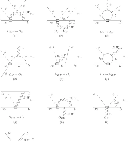
Fig. 2.3, where we show representative contributions to operator self-renormalization

and mixing among the various operators. The latter include mixing of all operators

into _O_{M, AD}(6) (a–c); mixing of _O_{M, AD}(6) , _O_{B, AD}(6) , and _O_{W, AD}(6) into _O(6)_{V , AD}_˜ (d, e); and mixing between the four-fermion operators and the magnetic moment operators (f,

g). Representative self-renormalization graphs are given in Fig. 2.3(h–j). As noted in

[68], the mixing of the the four-fermion operators into _O_{M, AD}(6) contains three powers of the lepton Yukawa couplings and is highly suppressed. In contrast, all other mixing

contains at most one Yukawa insertion.

Working to first order in the fAA we find a total of 59 graphs that must be computed, not including wavefunction renormalization graphs that are not shown.

Twenty-two of these graphs were computed by the authors of [69] in their

analy-sis of the mixing between _O_{M, AD}(6) and the magnetic moment operators. Here, we compute the remaining 37. As in [69], we work with the background field gauge

[79] in d = 4₋2 spacetime dimensions. We renormalize the operators using mini-mal subtraction, wherein counterterms simply remove the divergent 1/ terms from the one-loop amplitudes. The resulting renormalized operators _O_jR(6) are expressed in terms of the unrenormalized operators _O(6)_j as

OjR(6) = X

k

Z_jk−1ZnL/2

L Z nφ/2

φ O

(6)

k = X

k

Z_jk−1_O_k(6)₀ , (2.18)

where

Oj(6)0 =Z

nL/2

L Z nφ/2

φ O

(6)

j (2.19)

are theµ-independent bare operators; Z_L1/2 and Z_φ1/2 are the wavefunction renormal-ization constants for the fields LA and φ, respectively; nL and nφ are the number of LH lepton and Higgs fields appearing in a given operator; andZ−1

jkZ nL/2

L Z nφ/2

φ are the

counterterms that remove the 1/ divergences.

Since the bare operators_O(6)_j₀ do not depend on the renormalization scale, whereas the Z_jk−1 and the _O(6)_jR do, the operator coefficients C6

(41)

RG equation for the operator coefficients: µ d dµC 6 j + X k

C_k6 γkj = 0 (2.20)

where

γkj = X ` µ d dµZ −1 k`

Z`j . (2.21)

is the anomalous dimension matrix. We obtain7 _γ

jk=                 

−3(α1−3α₂) 16π

3α₁

8π −6α1(α1+α2) −

9α₁f∗

AA

8π −

9α₁f_AA

4π −

9α₁f_BB

2π

9α₁f_BB

4π

9α₂

8π

3(α1−3α2)

16π 6α2(α1+ 3α2)

27α₂f∗

AA

8π −

9α₂f_AA

4π −

9α₂f_BB

2π

9α₂f_BB

4π

0 0 9(α1+3α2)

16π −

3λ

2π2 0 0 0 0

0 0 9α2fAA

8π −

3f_AAλ

8π2

3α1

4π 0 0 0

−3fAA∗

128π2 −

f∗

AA

128π2 0 0

3(3α₁₋α₂)

8π 0 0

−3fBB∗

128π2 −

f∗

BB

128π2 0 0 0

3(α₁+α₂) 8π

3(α₁₋α₂) 4π

0 0 0 0 0 3(α1−α₂)

4π

3(α₁+α₂) 8π                  (2.22)

where the αi = gi2/(4π) and λ is the Higgs self coupling defined by the potential

V(φ) =λ[(φ†_φ₎₋_v2_/_2]2_.

Using this result for γij and the one-loop β functions for α1, α2, and the lepton Yukawa couplings, we solve the RG equations to determine the operator coefficients

C6

k(µ) as a function of their values at the scale Λ. As in [69] we find that the the running of the gauge and Yukawa couplings has a negligible impact on the evolution

of the C6

k(µ). It is instructive to consider the results obtained by retaining only the leading logarithms ln(µ/Λ) and terms at most first order in the Yukawa couplings.

7_{The term in}_γ

33 proportional toλdiffers from that of [69], which contains an error. However,

(42)

+... φ φ φ φ φ φ (b)

OV˜ →OM OF→OM

OF +... φ φ +... φ +... φ φ φ φ +... φ φ +... φ +... (d)

(g) (e) (h) (c) (f) (i) OB,W

OB,W _→OF

OB,W _→O_V˜

OM _→OV˜

OV˜

OF →OB,W νR

νR L L

lR

W

lR L

νR L νR L lR νR L

L lR

W

lR

νR L νR νR

+... B, W

L

B, W W

B

lR

νR L

L lR

B, W

(j)

lR L

B, W φ

+... φ

φ φ

OB,W →OM (a)

νR L

B, W

[image:42.612.112.536.56.525.2]

B, W

(43)

φ _φ φ φ _φ φ φ B, W B, W B, W (c) (b) (a) L

lR lR L lR L

L

νR νR L νR L

[image:43.612.118.531.204.642.2]

+...

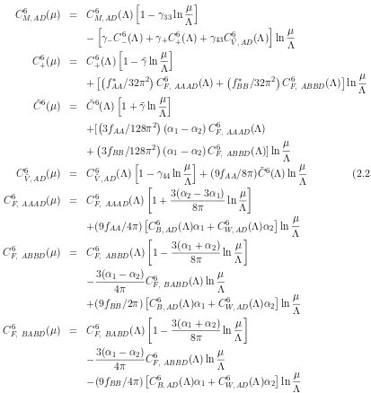
Figure 2.4: Two-loop graphs for the mixing of then = 6 operators. Only representive graphs for the mixing of the four-fermion operators_O(6)_{F, ABCD} into _O(6)_{M, AD} are shown.

We find

C_{M, AD}6 (µ) = C_{M, AD}6 (Λ)h1₋γ33lnµ Λ i

−hγ−C−6(Λ) +γ+C

6

+(Λ) +γ43C_{V , AD}6˜ (Λ)

i lnµ

Λ

C₊6(µ) = C₊6(Λ)h1₋˜γlnµ Λ i

+ f∗

AA/32π2

C_{F, AAAD}6 (Λ) + f∗

BB/32π2

C_{F, ABBD}6 (Λ)lnµ Λ ˜

C6(µ) = C˜6(Λ)h1 + ˜γln µ Λ i

+[ 3fAA/128π2

(α1 ₋α2)C_{F, AAAD}6 (Λ) + 3fBB/128π2

(α1₋α2)C_{F, ABBD}6 (Λ)] ln µ Λ

C_{V , AD}6˜ (µ) = C_{V , AD}6˜ (Λ)

h

1₋γ44lnµ Λ i

+ (9fAA/8π) ˜C6(Λ) ln

µ

Λ (2.23)

C_{F, AAAD}6 (µ) = C_{F, AAAD}6 (Λ)

1 + 3(α2−3α1)

8π ln

µ

Λ

+(9fAA/4π)

C_{B, AD}6 (Λ)α1+C_{W, AD}6 (Λ)α2lnµ Λ

C_{F, ABBD}6 (µ) = C_{F, ABBD}6 (Λ)

1₋ 3(α1+α2) 8π ln

µ

Λ

−3(α1₄−_π α2)C_{F, BABD}6 (Λ) lnµ Λ +(9fBB/2π)

C_{B, AD}6 (Λ)α1+C_{W, AD}6 (Λ)α2lnµ Λ

C_{F, BABD}6 (µ) = C_{F, BABD}6 (Λ)

1₋ 3(α1+α2) 8π ln

µ

Λ

−3(α1−α2)

4π C

6

F, ABBD(Λ) ln

µ

Λ

−(9fBB/4π)

(44)

where

C±6(µ) ≡ CB, AD6 (µ)±CW, AD6 (µ) ˜

C6(µ) _≡ α1CB, AD6 (µ)−3α2CW, AD6 (µ) (2.24)

γ± ≡ (γ13±γ23)/2

˜

γ _≡ 3(α1+ 3α2)/16π .

We note that the combination of coefficients C6

+(v) enters the neutrino magnetic

moment. Its RG evolution was obtained in [69] to zeroth order in the Yukawa

cou-plings; here we obtain the corrections that are linear infAAandfBB. The correspond-ing contributions to the neutrino mass matrix δmAD

ν and magnetic moment matrix

µAD

ν are then given by

δmAD_ν = ₋

v3

2√2Λ2

C_{M, AD}6 (v) (2.25)

µAD ν

µB

= ₋4√2mev Λ2

ReC₊6(v) . (2.26)

From Eqs. (2.23), (2.25), and (2.26) we observe that to linear order in the lepton

Yukawa couplings, C6

M, AD(µ) receives contributions from the two magnetic moment operators and _O(6)_V_˜ but not from the four fermion operators. This result is consis-tent with the result obtained by the authors of [68], who computed one-loop graphs

containing the four-fermion operators of Eq. (2.1) using massive charged leptons and

found that contributions to mν ∝ m3`. In the effective theory used here, the latter result corresponds to a one-loop computation with three insertions of the Yukawa

in-teraction. However, mixing with _O(6)_V_˜ was not considered in [68], and our result that this operator mixes with _O_{M, AD}(6) to linear order in the Yukawa couplings represents an important difference with the former analysis.

We agree with the observation of [68] that the four fermion operators can mix

[image:44.612.219.426.61.157.2]

(45)

and Z0 _{bosons that correspond in our framework to the diagrams of Fig. 2.4a. We}

observe, however, that the two-loop constraints will be we