Dimensionality Reduction in
Non-Parametric Conditional Density Estimation
with Applications to Nonlinear Time Series
A thesis submitted for the degree of
Doctor of Philosophy
by
Roy Rosemarin
Department of Statistics
The London School of Economics
This work was carried out under the supervision of
Professor Qiwei Yao
Declaration
I certify that the thesis I have presented for examination for the MPhil/PhD degree of the London
School of Economics and Political Science is solely my own work other than where I have clearly
indicated that it is the work of others (in which case the extent of any work carried out jointly by me
and any other person is clearly identified in it).
The copyright of this thesis rests with the author. Quotation from it is permitted, provided that full
acknowledgement is made. This thesis may not be reproduced without my prior written consent.
I warrant that this authorisation does not, to the best of my belief, infringe the rights of any third party.
Nonparametric methods of estimation of conditional density functions when the
dimen-sion of the explanatory variable is large are known to su¤er from slow convergence rates due
to the ‘curse of dimensionality’. When estimating the conditional density of a random
vari-ableY given randomd-vectorX, a signi…cant reduction in dimensionality can be achieved,
for example, by approximating the conditional density by that of aY given TX, where the
unit-vector is chosen to optimise the approximation under the Kullback-Leibler criterion.
As a …rst step, this thesis pursues this ‘single-index’ approximation by standard kernel
methods. Under strong-mixing conditions, we derive a general asymptotic representation
for the orientation estimator, and as a result, the approximated conditional density is shown
to enjoy the same …rst-order asymptotic properties as it would have if the optimal was
known. We then proceed and generalise this result to a ‘multi-index’approximation using
a Projection Pursuit (PP) type approximation. We propose a multiplicative PP
approx-imation of the conditional density that has the form f(yjx) = f0(y)QMm=1hm y; Tmx ,
where the projection directions m and the multiplicative elements, hm,m= 1; :::; M, are
chosen to minimise a weighted version of the Kullback-Leibler relative entropy between the
true and the estimated conditional densities. We …rst establish the validity of the
approx-imation by proving some probabilistic properties, and in particular we show that the PP
approximation converges weakly to the true conditional density as M approaches in…nity.
An iterative procedure for estimation is outlined, and in order to terminate the iterative
estimation procedure, a variant of the bootstrap information criterion is suggested. Finally,
the theory established for the single-index model serve as a building block in deriving the
asymptotic properties of the PP estimator under strong-mixing conditions. All methods
are illustrated in simulations with nonlinear time-series models, and some applications to
prediction of daily exchange-rate data are demonstrated.
I would like to take this opportunity to thank some of the people who have helped me
bring this thesis to its completion.
I am deeply indebted to Professor Qiwei Yao for introducing me to the topic of
dimen-sionality reduction and directing me throughout this research. Thanks to his willingness to
share from his own insightful perspective, but also his readiness to allow me to develop my
research directions independently, this research thesis took shape. I am sincerely grateful
to him for his invaluable and constructive criticism during my thesis writing and for his
encouragement at all stages of my work.
I am most grateful to Professor Yingcun Xia and Professor Piotr Fryzlewicz for willingly
accepting to be part of the examination committee and to evaluate this thesis. Their
comments made this thesis much more interesting in terms of theoretical and numerical
results, and hopefully more reader-friendly.
A very special thanks goes to my beloved partner, Georgia Ladbury, for her ongoing
personal support and encouragement. I very much appreciate her e¤ort and kind assistance
in proofreading this entire thesis and correcting my grammatical errors. All remaining
errors are my own. But more than anything else, I am thankful for her belief in me, which
spurred me on towards the completion of this thesis.
This thesis would not have been possible without the …nancial support provided to me
by more than one party. I am very grateful to the London School of Economics and the
Department of Statistics, who provided me with generous …nancial support and facilities to
carry my research throughout my Ph.D. studies. I very much appreciate all other friends
and family, who were willing to support me …nancially from time to time. These obviously
include my parents, Yehuda and Margalit Rosemarin, my partner, Georgia Ladbury, and
also my close friend, Michael Yosipov.
I am very thankful to Ian Marshall, the Research Administrator of the Department of
Statistics at the London School of Economics, for the ongoing support and kind assistance
that goes beyond simply “doing his job”.
and belief in me.
Roy Rosemarin
February 2012
Abstract . . . i
Acknowledgments . . . ii
1 Introduction 1 1.1 Motivation and Objectives . . . 1
1.2 Thesis Outline and Research Contributions . . . 3
2 Semiparametric Estimation of Single-Index Conditional Densities for De-pendent Data 7 2.1 Introduction . . . 7
2.2 Model and Estimation . . . 8
2.3 Asymptotic Results . . . 12
2.4 Implementation and Simulations . . . 19
2.5 Appendix A - Proofs of the Theorems . . . 32
2.6 Appendix B - Technical Lemmas . . . 49
3 Projection Pursuit Conditional Density Estimation 62 3.1 Introduction . . . 62
3.2 The Projection Pursuit Approximation . . . 64
3.3 Properties of the Optimal Projections . . . 70
3.4 Estimation Methodology and Algorithm . . . 81
3.5 Asymptotic Theory . . . 88
3.6 Information Criterion Stopping Rule . . . 96
3.7 Numerical study . . . 101
4 Discussion 130
References 137
Chapter 1
Introduction
1.1 Motivation and Objectives
Conditional probability density functions (c.p.d.f.) provide complete information on the
relationship between independent and dependent random variables. As such, they play a
pivotal role in applied statistical analysis. Applications include regression analysis (Yin
and Cook 2002), interval predictions (Hyndman 1995, Fan and Yao 2003), sensitivity to
initial conditions in nonlinear stochastic dynamic systems (Yao and Tong 1994, Fan, Yao
and Tong 1996), quantiles estimation and measuring Value-at-Risk (Engle and Manganelli
2004, Wu, Yu and Mitra 2008), and asset pricing (Aït-Sahalia 1999, Engle 2001), among
others.
If the conditional density has a known parametric form, then the estimation of the
c.p.d.f. reduces to estimation of a …nite number of parameters. In particular, if the
c.p.d.f. is assumed to be Gaussian then it can be fully characterised by a model for the
conditional mean and the variance, e.g. ARMA and GARCH time-series models. However,
it is often the case that probability densities are characterised by asymmetry, heavy-tails,
multimodality, and possibly other a priorily unknown features. Furthermore, even for
known parametric models, c.p.d.f. of nonlinear systems may be hard to derive analytically
(see Fan and Yao 2003). In such cases when the form of the c.p.d.f. is unknown or hard
to derive, adopting a nonparametric approach can be bene…cial.
In this thesis we consider a nonparametric estimation of the c.p.d.f. fYjX(yjx) of a
a purely nonparametric approach may su¤er from poor performance due to the ‘curse of
dimensionality’and the ‘empty space phenomenon’(see Silverman 1986, Section 4.5).
In order to overcome this ‘curse’, a vast number of techniques have emerged in the
liter-ature for reducing the dimensionality of the problem, without losing too many of the main
characteristics of the data. These include Principal Component Analysis (see Jolli¤e 2002),
Factor Analysis (see Gorsuch 1983), Independent Component Analysis (Comon 1994)
addi-tive and generalised-addiaddi-tive models (Hastie and Tibshirani 1990, Linton and Nielsen 1995,
Horowitz and Mammen 2007), single index models (Powell, stock and Stoker 1989, Härdle
and Stoker1989, Ichimura 1993, Delecroix, Härdle and Hristache 2003), inverse regression
estimation methods (Li 1991, Cook and Weisberg 1991), MAVE and OPG methods (Xia et
al 2002, see also Xia 2007, 2008), and successive direction estimation (Yin and Cook 2005,
Yin, Li and Cook 2008), among many others. Dimension reduction techniques aimed
di-rectly at estimation of conditional densities were studied by Hall, Racine and Li (2004) and
Efromovich (2010), where dimensionality reduction is achieved by attenuation of irrelevant
covariates. Hall and Yao (2005) and Fan et al (2009) o¤ered a single-index approximation.
This aim of this thesis is to contribute to this line of research by suggesting two related
approximation techniques of the c.p.d.f., based on the information gained by univariate
projections of the X-data. In addition, by allowing the data to be stationary
strong-mixing, the suggested approximations are shown to be applicable for dependent data, and
in particular to the estimation of predictive densities in time-series.
De…nition: A stationary processfZt;t= 0; 1; 2; :::g is said to be strong-mixing or
alpha-mixing if
k= sup
A2F0
1; B2Fk1
jP(A)P(B) P(AB)j !0 as k! 1;
whereFij denotes the -algebra generated by fZt;i t jg. We callf kgk2N the mixing
coe¢ cients.
strong-mixing under some mild conditions (cf. Pham and Tran 1985, Carrasco and Chen
2002, Davis and Mikosch 2009), and our method can be applied to these series when the
assumption of Gaussianity is not applicable. For a general univariate strong-mixing series
fztgnt=1+d+k 1;let
yt=Zt+d+k 1; xt= (Zt+d 1; :::; Zt)T ; t= 1; :::; n:
ThenfYjXt(ytjxt) provides ak-steps ahead conditional density based on the d-lagged
vec-torxt, which allows generalising standard time-series models to possibly nonlinear or
non-gaussian processes.
1.2 Thesis Outline and Research Contributions
In the second chapter of the thesis, we suggest approximating the conditional densityf(yjx)
by f yj Tx , the conditional density of Y given TX= Tx, where the orientation is a
scalar-valued d-vector that minimises the Kullback-Leibler (K-L) relative entropy,
Elogf(yjx) Elogf yj Tx :
The approximated conditional densityf yj Tx is estimated nonparametrically by a kernel estimator. In doing so, our approach provides a low dimensional approximation of the
conditional density which is optimal under the Kullback-Leibler criterion.
The approach of using the K-L relative entropy for estimation of orientation has been
utilised by Delecroix, Härdle and Hristache (2003) in single-index regression, Yin and Cook
(2005) for dimension reduction subspace estimation, and by Fan et al (2009), who similar
to us, dealt with conditional densities. Yin and Cook (2005) discuss several equivalent
presentations of the K-L relative entropy and they show relations to inverse regression,
maximum likelihood and other ideas from information theory.
by allowing the data to be stationary strong-mixing, as discussed in the previous section.
As a second contribution, we derive a general asymptotic representation for the di¤erence
between the orientation estimatorband the unknown optimal orientation 0 that is equal
to a sum of zero-mean asymptotic Gaussian components withpn-rate of convergence and
two other, stochastic and deterministic, components. The representation holds for kernels
of any order, while the asymptotically dominant terms are determined by the order of
kernels in use and the choice of kernel bandwidths.
Kernels of high-order bene…t from reduced asymptotic bias in the estimation, yet they
take negative values and thus often produce negative density estimates. An investigation
by Marron and Wand (1992) of higher order kernels for density estimation concluded that
the practical gain from higher order kernels is often absent or insigni…cant for realistic
sample sizes (see also Marron 1992 for graphical insight into the e¤ectiveness of high-order
kernels). Our proposed procedure allows estimating 0 with high-order kernels, while then
estimating the conditional density with non-negative second-order kernels.
The method is illustrated in simulations with nonlinear time-series models, and an
application to prediction of daily exchange-rate volatility is demonstrated.
In Chapter 3 of the thesis, we proceed and generalise the result of Chapter 2 to a
‘multi-index’approximation using a Projection Pursuit type approximation. More precisely,
mo-tivated by the Projection Pursuit Density Estimation (PPDE) of Friedman, Stuetzle and
Schroeder (1984), we propose a multiplicative projection pursuit approximation of the
con-ditional density that has the formf(yjx) =f0(y)QMm=1hm y; Tmx , where the projection
directions m and the multiplicative elements, hm, m = 1; :::; M, are chosen to minimise
a weighted version of the Kullback-Leibler relative entropy between the true and the
es-timated conditional densities. In particular, the single-index approximation of Chapter 2
can be seen as a private case of the projection pursuit approximation whenM = 1. Indeed,
in Chapter 3, the single-index approximation serves as a theoretical building block for the
projection pursuit approximation, which allows us to derive the asymptotic properties of
Other ‘multi-index’ extensions of the single-index c.p.d.f. approximation have been
proposed in the literature by Xia (2007) and by Yin, Li and Cook (2008). Both these
papers aim to estimate the central dimension reduction subspace spanned by the column
of d q orthogonal matrix B; q d; such that f(yjx) = f yjBTx (see Cook 1998).
However, while these papers o¤er a method to estimate the central dimension reduction
subspace, estimation of the c.p.d.f. can still be cumbersome to implement, even in the
reduced subspace, which may still be of high-dimension. The projection pursuit method
o¤ers a di¤erent generalisation of the single-index c.p.d.f. approximation, in that it
at-tempts to approximate the c.p.d.f. directly by a multi-index approximation, while it does
not necessarily produce an e¤ective estimate of the dimension reduction subspace.
Un-fortunately, the ‡exibility of the Projection Pursuit approximation comes at the cost of
interpretability, as the obtained estimates for M, m’s and hm’s can be hard to interpret
in practice.
In the third chapter, we …rst establish the validity of the projection pursuit
approxima-tion by proving some probabilistic properties, and in particular we show that the projecapproxima-tion
pursuit approximation converges weakly to the true conditional density asM approaches
in…nity. Similar properties have been proved to hold for the PPDE by Friedman, Stuetzle
and Schroeder (1984) and Huber (1985). However, some adaptations of their arguments
are required to account for the di¤erent nature of the problem discussed in this thesis and
the modi…ed Kullback-Leibler criterion for c.p.d.f’s, which is in use.
After establishing the theoretical approximation, an iterative procedure for estimation is
outlined, based on similar principles as for the projection pursuit density estimation.
How-ever, due to the nature of the problem, there is no need to incorporate cumbersome Monte
Carlo samplings as in the projection pursuit density estimation, rendering our method
sim-ple and computationally undemanding even for very large datasets. In order to terminate
the iterative estimation procedure, a variant of the bootstrap information criterion is
sug-gested that has the advantage of avoiding the need to solve an optimisation problem for
asymptotic properties of the proposed projection pursuit estimator under strong similar
mixing conditions.
Finally, the projection pursuit method is illustrated in simulations with nonlinear
time-series models, and an application to prediction of daily exchange-rate data is demonstrated.
Chapter 4 brie‡y concludes and summarises the achieved results and possible directions
Chapter 2
Semiparametric Estimation of Single-Index
Conditional Densities for Dependent Data
2.1 Introduction
In this chapter, we consider an approximation of the conditional density fYjX(yjx) by
fYj TX yj Tx , the conditional density ofY given TX= Tx, where the orientation is
a scalar-valuedd-vector that minimises the Kullback-Leibler (K-L) relative entropy,
ElogfYjX(yjx) ElogfYj TX yj
Tx : (2.1)
The approximated conditional density fYjTX yj Tx is estimated nonparametrically by
a kernel estimator. In doing so, our approach provides a low dimensional ‘single-index’
approximation of the conditional density which is optimal under the Kullback-Leibler
cri-terion.
In the single-index regression model (see Ichimura 1993) it is typically assumed that
Y =g TX +", wheregis some link function and"is a noise term such thatE("jX) = 0. Our methodology di¤ers from this regression model by aiming for the most informative
projection TX of X to explain the conditional density of Y given X, rather than just
the conditional mean. However, that is not to say that the true conditional distribution
of YjX is assumed to be the same as that of Yj TX. The method aims to provide the
optimal single-index conditional density approximation possible for a generalfYjX(yjx).
a result by Gao and King (2004), who established a moment inequality for degenerate
U-statistics of strongly dependent processes, given in Lemma 2.6.4.
De…nition 2.1.1 A U-statistic of general order m 2 is a random variable of the form
Un=
X
1 i1<:::<im n
H(Zi1; :::; Zim); (2.2)
where H is a real-valued function, symmetric in itsm arguments, and X1; :::; Xn are
sta-tionary random variables (or vectors). If for any …xed zi2; :::; zim we have
E(H(Zi1; zi2; :::; zim)) = 0;
then the U-statistic is said to be degenerate.
U-statistics play a key role in the literature in deriving the asymptotic properties of
semiparametric index-models for independent observations (e.g. Powell, Stock, and Stoker
1989, Delecroix, Härdle and Hristache 2003 and Delecroix, Hristache and Patilea 2006),
and in order to extend this theory to dependent observations we rely heavily on Gao and
King’s (2004) result.
The outline for the rest of the Chapter is as follows. Section 2.2 states the model’s
general setting and estimation methodology; Section 2.3 contains the assumptions and
main theoretical results; and Section 2.4 presents a numerical study with three simulated
time-series examples and exchange-rate volatility series. The proofs of the main theorems
are given in Section 2.5, while some other technical lemmas are outlined in Section 2.6.
2.2 Model and Estimation
Letfyj; xjgnj=1be strictly stationary strong-mixing observations with the same distribution
as(Y; X), whereY is a random scalar andX is a randomd-vector. Our aim is to estimate
the conditional densityfYj TX yj Tx ofY given a randomd-vector TX= Tx;where is
relative entropy does not depend on , minimising K-L relative entropy is equivalent to
maximising the expected log-likelihoodElogfYj TX yj Tx . Clearly, the orientation is
identi…able only with regards to its direction and sign inversion, and we therefore consider
unit-vectors that belong to the compact parameter space
=n 2Rd: T = 1; 1 c >0
o
;
where 1 is the …rst element of the orientation andc >0is arbitrarily small. For example,
if Yt is the k-step ahead observation of a time-series and Xt consists of d lagged values
of the series, then the constraint that 1 6= 0 represents the belief that the k-step ahead
observation depends on the most recent observed value.
In order to ensure the uniform convergence of our estimator, we need to restrict ourselves
to a compact subset of the support of Z = (Y; X) such that for any 2 the probability
densityfYjTX yj Tx is well de…ned and bounded away from0. Denote such a subspace
byS, and let alsoSX = x2Rd:9y s.t. (y; x)2S . Let 0 be the maximiser of expected
log-likelihood conditional onZ 2S, that is,
0 = arg max
2 ES logfYj TX Yj
TX ; (2.3)
where ES is the conditional expectation given Z 2 S. Note that the condition Z 2 S
should not have any signi…cant e¤ect on 0 if the subset S is large enough. For ease of
presentation, we shall assume that all observationsfyj; xjgnj=1 belong toS.
To estimate 0 one can maximise a sample version of (2.3). De…ne the orientation
estimator byb= arg max 2 L( ), whereL( )is the likelihood function
L( ) = 1
n
n
P
i=1
logfbYi
j TX yij
Tx
i bi: (2.4)
nonparametric kernel estimator
b
f i
Yj TX yij
Tx i =
b
f i
Y; TX yi; Tx
i
b
f TiX
Tx i
:
where fbY; TX y; Tx and fbTX Tx denote the standard kernel probability density
es-timates, whereas the superscript ‘ i’ indicates exclusion of the i0th observation from the
calculation, that is,
b
f i
Y;TX yi; Tx
i = f(n 1)hyhxg 1 P j6=i
K yj yi hy
K
T(x j xi)
hx
!
;
b
f TiX
Tx
i = f(n 1)hxg 1P j6=i
K
T(x j xi)
hx
!
;
wherehy; hx are bandwidths andK is a …xed, bounded-support, kernel function.
The exclusion of a single observation from the calculation should not have
asymp-totic e¤ect, but is mainly used for theoretical convenience, as it removes any extraneous
bias terms that may arise from reusability of data. While this ‘leave-one-out’formulation
becomes necessary when smoothing parameters are estimated along with the orientation
parameter (see Härdle, Hall, and Ichimura 1993), it has been widely used in the literature
for single-index modelling even when no estimation of smoothing parameter is involved (cf.
Powell, Stok, Stoker 1993, Ichimura 1993, Hall 1989). Note that adding the i0th
observa-tion, i.e. the j =i case, contributes a deterministic term of the form nh 1K(0) to each
density estimate, and therefore it may stabilise the …nite-sample performances as it ensures
that all density estimates are positive. On the other hand, adding the term nh 1K(0)to
each density estimate seems heuristic, and in general one may consider adding any
non-stochastic decaying term "n ! 0 to the density estimates with the purpose of ensuring
positivity. However, as this method can be very sensitive to the choice of "n, here we
applied a trimming operator for this purpose.
if observation (yi; xi) belongs to S it may still be the case that the kernel estimates
b
f i
Y; TX yi;
Tx
i , fbTiX
Tx
i rely on very few neighbouring observations, or even none,
and as a result these estimates may be close to zero and even non-positive when high-order
kernels are used. Including logfb i
YjTX yij
Tx
i in the computation of the likelihood
func-tion in such cases may have a drastic adverse e¤ect on the accuracy of the likelihood surface
estimates, and it is therefore preferable to trim such terms. Here, we adopted the following
simple data-driven trimming scheme, which works very well in practice (For alternative
trimming schemes, cf. Härdle and Stoker 1989, Ichimura 1993, Delecroix, Hristache and
Patilea 2006, Ichimura and Todd 2006 and Xia Härdle and Linton 2012). For a given
observation (yi; xi) and 2 , let
In;i =
8 > < > :
1; if minnfb i
Y; TX yi;
Tx
i ;fbTiX
Tx i
o
> a0n c;
0; otherwise,
for some small constants a0; c > 0. As In;i depends on it needs to be normalised to
account for the actual number of observations considered in the computation ofL( ), and hence we take
bi = In;i 1
n
Pn
i=1In;i : (2.5)
Thus, the trimming term bi is completely data-driven in the sense that it depends on
the set of observations, and in addition, it also depends on the value of the parameter ,
evaluated by the likelihood. However, it does not assume any prior knowledge or applying
a pilot estimation of 0. We show in appendix B that if c is su¢ ciently small, then bi
eventually equals to 1 for any large enough n with probability 1. Therefore, bi has no
asymptotic e¤ect on the method performance.
It is common in single-index regression models, that the optimal kernel’s bandwidths for
orientation estimation undersmooth the nonparametric estimator of the link function, in
the sense that these bandwidths have a faster rate of decay than the optimal rate for purely
indicates that a similar property arises in single-index conditional density estimation. It
is therefore the reason that a second stage of estimation is utilised whenfYj TX yj Tx is
estimated with the orientation estimate b and with optimal-rate bandwidths Hy and Hx
for nonparametric estimation. Moreover, the ‘two stages’ procedure allows estimating 0
with high-order kernels, while then estimating the conditional density with non-negative
second-order kernels.
Notice that although 0 is de…ned with respect to the true conditional density, it is
possible that the orientation estimator,b, will be more suitable to use at the second-stage with the same bandwidths and kernel functions as in the …rst-stage. However, this is likely
to happen only in very small sample sizes as the increase in accuracy achieved by using
optimal-rate bandwidths and non-negative kernels is likely to take e¤ect very quickly. For
further discussion, see also Hall (1989, pp. 583-4)
Our …nal c.p.d.f. approximation is obtained by using all observations in the calculation,
non-negative symmetric kernelsKe( );and with bandwidthsHy and Hx in place ofhy and
hx, that is
e
f
YjbTX yjb T
x =
1 nHyHx
Pn j=1Ke
yj y
Hy Ke
bT
(xj x)
Hx
1 nHx
Pn j=1Ke
bT
(xj x)
Hx
:
The following section presents the asymptotic properties of bandfe
YjbTX yjb T
x .
2.3 Asymptotic Results
We introduce some new notations that will be used throughout the section and in the
proofs. For a functiong( )of 2 and possibly of other variables, letrg( )andr2g( ) be the vector and matrix of partial derivatives ofg( ) with respect to , i.e.,
frg( )gk= @g( )
@ k
and r2g( ) k;l = @
2g( )
@ k@ l
Denote nowZ = (X; Y) and
( ) = ES
h
rlogfYjTX Yj TX rlogfY
j TX Yj
TX Ti; ( ) = ES
h
r2logfYj TX Yj TX
i
:
whereESis the conditional expectation givenZ 2S. For some small >0, de…ne also the
set S distant no further than >0from some y; Tx such that(y; x)2S and 2 .
The following assumptions are required to obtain the asymptotic results for the
orien-tation estimatorb.
(A1) The sequencefyj; xjgnj=1 is strictly stationary strong-mixing series with mixing
coe¢ cients that satisfy t A t with0< A <1 and 0< <1:
(A2) K( ) is a symmetric, compactly supported, boundedly di¤erentiable kernel.
(A3) The bandwidths satisfyhy; hx=o(1) andn1 hyhx! 1 for some >0.
(A4) For all 2 ; Y; TX has probability density fY; TX(y; t) with respect to
Lebesgue measure onS andinf(y;t)2S fY; TX(y; t)>0. fY; TX(y; t),E XjY =y; TX=t
andE XXTjY =y; TX =t are twice continuously di¤erentiable with respect to(y; t)2
S . Moreover, there is some j such that for allj > j and y1; Tx1 ; yj; Txj 2S the
joint probability density of y1; Tx1; yj; Txj is bounded.
(A5) For the trimming operator, we require that a0; c > 0 and nc h2y+h2x = o(1)
and n1 2c hyhx! 1 for some >0.
(A6) For all 2 ; ES logfYjTX is …nite and it has a unique global maximum 0
that lies in the interior of .
We further require that K( ) is ap’th-order kernel function, such that
Z
ujK(u)du= 0 for j= 1; :::; p 1; and
Z
upK(u)du6= 0;
forp 2. We then make the following assumptions.
(A7)K( )isp’th-order kernel withp 2, and it is three times boundedly di¤erentiable.
(A9)fY; TX(y; t)andE XjY =y; TX =t andE XXTjY =y; TX =t are(2 +p)
-times continuously di¤erentiable with respect to(y; t)2S :
Conditions (A1)-(A6) are needed for uniform consistency of the log-likelihood function
on S, and therefore for consistency ofb. In particular, condition (A1) allows the data to come from a strong-mixing process. As an example, ARMA, GARCH and stochastic
volatility processes satisfy condition (A1) (cf. Pham and Tran 1985, Carrasco and Chen
2002, Davis and Mikosch 2009). Condition (A2) requires that K( ) is symmetric and
therefore it is of second-order at the least. Condition (A3) on the bandwidths is needed to
obtain uniform convergence of the kernel density estimators. In condition (A4), the bound
on the joint probability density of TX1; Y1; TXj; Yj may not hold for j j , which
allows components of X1 and Xj to overlap for some small j’s, as in the case where Xt
consists of multiple lags ofYt. For example, ifxt= (yt 1; :::; yt d)T ford 2then the joint
probability density of Y0; TX0; Yj; TXj is unbounded forj < dbecause the components
of X0 and Xj overlap. Condition (A5) for the trimming operator terms is derived from
Lemma 2.6.5 in the appendix. (A6) is an identi…ability requirement for 0. In the case
whereES logfYj TX has more than a single global maximum, 0 can be any one within
the set of maxima points, and our asymptotic results will still apply as long as this 0 is a
local maximum in a small neighbourhood. Note that in that case, the choice of 0 within
the set of optimum points is not crucial as long as the approximation of fYjX(YjX) is
concerned. Conditions (A7)-(A9) are stronger versions of (A2)-(A4) and are needed for
the derivation of the rate of consistency of b. In these conditions, the order of the kernel
function K( ) is set to p 2, which has to be an even number if K( ) is a symmetric
by (A2). Kernels of high-order may take negative values, and thus they often produce
negative density estimates. However, the trimming scheme, introduced in Section 2.2, is
designed to trim non-positive estimates from the log-likelihood calculation, and therefore
any potential problems caused by non-positive density estimates are avoided. Condition
(A8) discusses rate of decay for the bandwidths. For example, if both bandwidths hy; hx
The following theorem, proved in Section 2.5. shows the consistency ofb: Theorem 2.3.1 Let (A1)-(A6) hold. Then as n! 1
b!p 0:
As an implication of Theorem 2.3.1 and the fact that both 0 andbare unit-vectors, it
follows from a simple geometric argument that the di¤erenceb 0 can be approximated
up to …rst-order asymptotics by b?, the projection of b into the plane orthogonal to 0,
i.e.,
b 0=b?+op b 0 .
Since fYj TX Yj TX depends only on the direction of , then for any vector 2Rd we
get that both vectorrlogfYjTX Yj TX and the column (row) space spanned by matrix r2logfYjTX yj Tx are perpendicular to . Indeed, this can also be seen directly from
Lemma 2.6.1 in appendix B. Note, however, that by conditions (A6) and (A9) there is
a generalised inverse of ( 0), denoted ( 0) , that is well de…ned in the perpendicular
space to 0 (cf. Theorem 3.1 of White 1982). Let now
V ( 0) = ( 0) ( 0) ( 0) :
The next theorem gives a general second-order asymptotic representation forb 0.
Theorem 2.3.2 Let (A1)-(A10) hold. Then
b 0 =n 1=2V ( 0)1=2Z+Op n2 hyh3x 1=2
+O(hpy+hpx);
where Z is asymptotically normal N(0; I) random d-vector and >0 arbitrarily small.
Similar results to Theorems 2.3.1 and 2.3.2 were derived by Delecroix, Härdle and
observations and fourth-order kernels, and they obtained
p
n b 0 !N(0; V ( 0)):
Yin and Cook (2005) also dealt with a similar model for the purpose dimension reduction
subspace estimation, and they derived consistency ofbunder independence.
Fan et al (2009) were the …rst to suggest applying the Kullback-Leibler criterion to
a single-index approximation of the conditional density. They also assumed independent
observations and obtained
b 0 =Op n2 hyh3x 1=2
:
Thus, Theorems 2.3.1 and 2.3.2 extends these papers by allowing the data to be stationary
strong-mixing, and by o¤ering a general second-order asymptotic representation forbthat is holds for kernels of any order.
The proofs of Theorems 2.3.1 and 2.3.2 are given in Appendix A of the Chapter. The
idea of the proofs of is to look …rst at
L( ) =n 1
n
P
i=1
logfYj TX yij Txi ;
which is a version of the likelihoodL( )when conditional density estimates are replaced by the true conditional densities. Deriving the asymptotic properties ofL( )is straightforward
by the ergodic theorem and CLT for strong-mixing processes (see Fan and Yao 2003,
Proposition 2.8 and Theorem 2.21).
At a second step in the proofs, we look at the di¤erenceL( ) L( ). By Lemma 2.6.5, all trimming-terms,bi,i= 1; :::; n, de…ned in (2.5), are eventually equal to 1 for any large
enough n with probability 1. Therefore, we can consider n to be large enough so bi 1
and
L( ) L( ) =n 1
n
P
i=1
log fb i
Yj TX yij Tx
i
.
For Theorem 2.3.1, it is then su¢ cient to prove that
sup
2 jL
( ) L( )j=op(1):
In the proof of Theorem 2.3.1, the main e¤ort is in the establishment of an asymptotic
bound for the di¤erence
rL b rL b : (2.6)
We write this di¤erence as a sum of few U-statistic terms. The main idea in the derivation
is to perform the Hoe¤ding’s decomposition on the U-statistic terms (Lemma A, pp. 178
in Ser‡ing 1980), and then apply the result for degenerate U-statistics of strong-mixing
processes by Gao and King (2004, Lemma C.2). We then manage to establish a uniform
bound for (2.6) over a shrinking neighbourhood of 0, in the sense that !p 0 implies
that
rL( ) rL( ) =Op n2 hyh3x 1=2
+O(hpy+hxp) +op( 0): (2.7)
Nolan and Pollard (1987) and Sherman (1994) developed a general uniform convergence
theory for U-statistics, and some applications include Ichimura (1995), Zheng (1998) and
Wang (2006). However, these results were obtained under assumption of independence,
while as far as we are aware, there is no general theory for uniform convergence of
U-statistics under mixing conditions. In the proof of Theorem 2.3.1, the property (2.7) is
achieved using a Lipschitz continuity property of the kernel functions in a similar manner
to Theorem 2 of Hansen (2008), see also the proof of Lemma 2.6.3 in Appendix B.
Theorem 2.3.2 implies that the choice of bandwidth hx has a greater impact on the
rate of convergence of b than that of the bandwidth hy. This is due to the fact the
orientation vector, which appears within the kernel density estimates, is related to the X
variable through the functionK T(xj xi)
hx . In particular, the symmetry betweenhx and
hy breaks when considering the score function rL( ), as one gets an additional factor of
It is clear from this theorem that forbto bepn-consistent estimator of 0, one needs
n2 hyh3x 1=2
n 1=2 and hpy+hpx n 1=2: (2.8)
However, it is easy to see that both conditions cannot be satis…ed if p= 2, and hence the
p
n-convergence rate is not achieved in that case (cf. Remark 2 of Fan et al 2009), although
the convergence rate can still become arbitrarily close topn. By increasing the order of the kernel top= 4, the condition (2.8) can be ful…lled underhy; hx n 1=2p andhyh3x n 1,
and if the two last inequalities are strict, then the Theorem implies asymptotic normality
of the estimate.
The asymptotic expression given by Theorem 2.3.2 at the limit ! 0 suggests that
the optimal bandwidthshy and hx have both the asymptotic raten 1=(p+2), wherepis the
kernel’s order. Taking p = 2, for example, we have that the optimal bandwidths are of
asymptotic ordern 1=4. This optimal rate re‡ects undersmoothing of the kernel estimator,
which is a typical requirement in many single-index models.
As an immediate consequence of Theorems 2.3.1 and 2.3.2, we get that under
appropri-ate choice of bandwidths,bcan converge fast enough to 0so thatfeY
jbTX yjb T
x estimates
fYj T 0X yj
T
0x with the same …rst-order asymptotic properties as if 0 was known. The
Theorem below formalises this idea.
Theorem 2.3.3 Let (A1)-(A10) hold and HyHx=hyh3x = o n1 for some > 0 and
HyHx h2yp+hx2p = o n 1 . In addition let Ke be a symmetric, compactly supported,
boundedly di¤ erentiable kernel, and Hy; Hx =O n 1=6 and nHlnynHx =o(1):Then for any
>0;
sup
(y;x)2S
e
f
YjbTX yjb T
x fYj T 0X yj
T
0x =Op
lnn nHyHx
1=2!
: (2.9)
Notice that the exact rate of consistency for conditional density kernel estimator is
(nHyHx) 1=2 (Robinson 1983). The lnn term in the RHS of (2.9) is needed to get a
uniform rate of convergence by Lemma 2.6.2. This upper bound for the uniform rate of
also Fan and Yao 2003, Theorem 5.4). As far as we are aware, Bickel and Rosenblatt’s
result was not generalised to the dependent case. Nevertheless, we would expect this to be
the case for general stationary process under certain mixing conditions.
Theorem 2.3.3 is proved in Appendix A of the Chapter.
2.4 Implementation and Simulations
In this section, we discuss implementation of the proposed method and we examine its
…nite-sample properties over few simulated time-series models.
In all of the simulations we used the three-time di¤erentiable and IMSE optimal kernels
with support ( 1;1), derived by Müller (1984) and speci…ed below. The second-order
Müller’s kernel, also known as the Triweight kernel, is given foru2( 1;1)by
K(u) = 35=32 1 3u2+ 3u4 u6 ; (2.10)
and the fourth-order Müller’s kernel is given foru2( 1;1)by
K(u) = 315=512 3 20u2+ 42u4 36u6+ 11u8 :
For the estimation of the conditional densityfe
YjbTX yjb T
x we use only the non-negative
Triweight kernel.
In order to facilitate the implementation, we standardised xj = (xj1; :::; xjd) by
set-ting xj Sx1(xj x) and we standardised yj by setting yj (yj y)=sy, where x
and y are the vector and scalar sample means of fxjgnj=1 and fyjgnj=1; and Sx2 and s2y
are the d d-matrix and the scalar sample variances. This procedure allows us to
dis-regard scaling parameters and to apply the same smoothing parameter for each direction
of 2 , in accordance with Scott’s (1992) normal reference rule. Once the two-stage
estimation procedure was complete, the estimates of the orientation and the conditional
and fe
YjbTX yjb T
x fe
YjbTX yjb T
x =sy.
We now provide a brief discussion on the topic of bandwidths selection. Typical
band-widths selection methods proposed in the literature of single-index models usually su¤er
from heavy computational burden. Härdle, Hall, and Ichimura (1993) proposed to
op-timise the least squares criterion function over the orientation coe¢ cients as well as the
bandwidth. A related iterative procedure of alternately estimating the orientation and the
bandwidth was suggested by Xia, Tong, Li (1999). Fan and Gijbels (1995a,b) combined
goodness of …t and plug-in steps to achieve variable bandwidth. Fan and Yim (2004) and
Hall, Racine and Li (2004) discussed cross-validation techniques for bandwidth selection.
Hall and Yao (2005) utilised a bootstrap approach based on the linear model to choose a
bandwidth. Moreover, most of the mentioned methods require applying the algorithm to
any 2 , or at least to some pilot estimator of 0. The computational burden in such
methods may be particularly noticeable in models like ours, where the estimation requires
solving a numerical multivariate optimisation problem. In practice, however, various prior
numerical studies that we carried out with di¤erent selection rules for hy and hx
demon-strated that the orientation estimator is very robust to the choice of bandwidths as long as
the bandwidths are not too small. Motivated by the single-index regression algorithm of
Xia, Härdle, Linton (2012), we propose the following iterative procedure that successfully
reconciles e¤ective bandwidth selection with fast and robust numerical optimisation.
Step 0. Let b0 2 be any initial guess for 0, for exampleb 0
= (1;0; :::;0). Set also
a …nite sequences of decreasing bandwidths hiy = hix = ain 1=(p+2); i = 1; :::; I, where p
is the kernel-order and ai > 0 is a decreasing sequence such that the …rst bandwidths
notably oversmooth the unconditional density and the last one is chosen, e.g., by Scott’s
(1992) normal reference rule. In our simulations, we used a1; a2; :::; aI = (9;8; :::;3),
which yields good results. Set the iteration numberi= 1.
Step 1. Apply a multivariate variant of the Newton-Raphson method with
start-ing pointbi 1 to …nd a maximum log-likelihood estimate bi numerically based on
method (see Nocedal and Wright 2006, Chapter 6).
Step 2. Stop the procedure and use the estimate b=bi either if i=I or if a certain convergence criterion is met, i.e. if bi Tbi 1 >1 " for some small " > 0. Otherwise, set i i+ 1and hiy =hxi =ain 1=(p+2), and return to Step 1.
Note that since h1y = h1x = 9n 1=(p+2) are chosen to oversmooth the conditional
den-sity in the …rst iteration of estimation, the corresponding likelihood surface is thus
over-smoothed as well, and the optimisation algorithm is insensitive to the choice ofb0. On the other hand, if we simply use one step of maximization with only hy = hx = 3n 1=(p+2),
then the algorithm is very likely to converge to some local maximum, depending on the
starting pointb0 provided. Having said that, one needs to be aware that if the expected likelihood surface is truly multimodal, oversmoothing the likelihood surface may lead to
convergence of the procedure to a locally optimal parameter, rather than to a globally
optimal one.
For the second stage estimator of the conditional density, fe
YjbTX yjb T
x , Theorem
2.3.3 assumes the bandwidthsHy andHx do not change when the …t is carried out on the
data. However, in practice, if the variables Y and bTX have a nonuniform distribution,
a constant bandwidths may lead to problems caused by undersmoothing in some sparse
neighborhoods. In order to overcome this problem, the nearest neighbour bandwidth
es-timator chooses the bandwidths to ensure that su¢ cient amount data is contained in the
calculation. More speci…cally, the nearest neighbor bandwidth for a density estimate at
point z, given stationary observations z1; :::; zn, is computed as the distance from z to its
k0th nearest neighbour among z1; :::; zn(cf. Silverman 1986, Section 2.5, Loader 1999,
Sec-tion 2.2.1, Scot 1999, SecSec-tion 6.6). Thus, for example, in the tails of the distribuSec-tion, the
nearest neighbour bandwidth will be larger than in the centre of the distribution, and so
the sparsity problems in the tails are reduced. However, nearest neighbour estimates are
generally not probability densities as they do not necessarily integrate to one as the tails
of the estimate may approach zero very slowly (see Silverman 1986, Section 2.5).
Other alternative methods for adaptive bandwidth are typically more complicated,
such as the locally adaptive two-stage kernel estimator of Breiman, Meisel and Purcell
(1977), and the supersmoother algorithm of Friedman and Stuetzle (1982), which chooses
bandwidths based on a local cross validation method. Few other local goodness of …t
approaches for bandwidth selection are discussed in Chapter 11 of Loader (1999). However,
according to Loader (1999), these locally adaptive procedures work very well on problems
with plenty of data, obvious structure and low noise, while when the data structure is
not obvious, simpler methods of bandwidth selection are generally preferable. Moreover,
locally adaptive procedures are charachterised by tuning parameters, or penalties, and the
estimates can be quite sensitive to the choice of these parameters.
In our simulation study, we have considered at …rst an application of the nearest
neigh-bour procedure for the second stage of estimation by using the R statistical package ‘loc…t’
of Clive Loader. This package allows combining a …xed bandwidth with a nearest neighbor
bandwidth, such that the …nal bandwidth is determined as the maximum amongst both
components. An asymptotic analysis by Moore and Yackel (1977) suggest that the
para-meterkin the nearest neighbour estimator is linked to the bandwidthhin a nonparametric
kernel estimation byk=nhd. Hence, for our study, Scott’s (1992) normal reference rule for
bandwidth selection suggests using bandwidths that are taken as the maximum between
an 1=6 and the k0th nearest neighbour with parameter k = an5=6, where for Triweight
kernel (2.10) a 3. Nevertheless, after gaining some experience with the method, we
came to conclude that while the nearest neighbour method is more demanding in terms
of computational time, it o¤ered no signi…cant bene…t relatively to the …xed bandwidth
in terms of minimisingRM SP E in our Monte Carlo study or prediction of out-of-sample
conditional tail quantiles in a real-data example. In all of our simulations reported below,
we have therefore used …xed bandwidths according to Scott’s (1992) normal reference rule,
which suggests using bandwidths given byHy =Hx= 3n 1=6.
As with most other trimming schemes proposed in the literature (cf. Härdle and Stoker
Xia, Härdle and Linton 2012), our trimming method requires setting values for the
trim-ming parameters; these are a0 and c. Since the trimming factor (2.5) serves also as a
normalising factor, our method is expected to be relatively robust to the trimming
para-meters as long asa0n c is not too small such that any single observation may have a strong
e¤ect on the likelihood function value. At the same time, a good choice of values fora0and
cshould aim to trim only as few observations as possible, in the sense that the probability
that minnfY; TX yi; Txi ; f TX Txi
o
is smaller than a0n c is very low. In practice,
in all of our simulations, we used all observations in both stages of the estimation, and we
setbi to trim down only observations whose density estimates were lower than 0:001. The complexity of the proposed algorithm is calculated as follows. Computing the
likelihood has a computational complexity of O n2d , since it is calculated as a sum of
n(n 1) terms, j 6= i, where each term requires calculating the inner product of with
(xj xi). Note that each term also requires applying the kernel function which may take
some expensive computational time, and therefore it is generally recommended to choose
kernels of simple form (i.e., polynomials). The BFGS optimisation method is a hill-climbing
optimisation technique, and it requires O d2F(n; d) time per step of the optimisation
algorithm to optimise a system withdparameters, whereF(n; d)is the cost of calculating
the objective function (Nocedal and Wright 2006, Chapter 6). Thus, in our case, assuming
the number of steps of the BFGS optimisation algorithm is limited to a …nite number,
the computational complexity of …nding the MLE, b, using the the BFGS method is of
order O n2d3 . Similar considerations show that the computational complexity of the
second step of the estimation, i.e., calculatingfe
YjbTX yjb T
x , is of orderO(nd), which is
relatively insigni…cant.
In the simulations we used R 2.14.1 programme on a computer with 3.4ghz intel core
i7-2600 processor. In all of the examples considered below, the dimensionality of the problem
wasd= 4. The average computational times of the method (for a single estimation based
on Example 1 below) with dimension d = 4 and sample sizes n = 100;200;400 and 800
An R code PPCDE.txt for the calculations below is available at
http://personal.lse.ac.uk/rosemari/
For comparison, we also tested thedOP G method of Xia (2007)y. ThedOP G method
performs estimation the central dimension reduction subspace, and when it is exercised
with a one-dimensional central dimension reduction subspace, it can be applied for the
the …rst-stage estimation of the orientation vector. For the dOP G method the average
computational times of the method (for a single estimation based on Example 1 below)
with dimensiond= 4 and sample sizesn= 100;200;400and 800were1 sec;1 sec;2 secand
5 sec, respectively.
The performances of the proposed methods are demonstrated in the following three
examples of simulated time-series models.
Example 1. As a …rst example, we consider the linear AR(4) model
yt= 0:5
X4
j=1 0;jyt j+ 0:5 "t;
where T0 ( 0;1; ::; 0;4) = (3;2;0; 1)=
p
14 and "t are i.i.d. N(0;1).
Example 2. In the next example we consider the nonlinear AR(4) model
yt=g
X4
j=1 0;jyt j + 0:5 "t;
where g(u) = exp 0:4 2u2 u , T0 ( 0;1; ::; 0;4) = (1;2; 1;0)=
p
6, and the "t are as
in Example 1.
Example 3. Finally we would like to examine how the method works where the optimal projection T0X is related to higher moments ofX. For the third example, we consider the
nonlinear ARCH(4) model
yt=g
X4
j=1 0;jyt j "t;
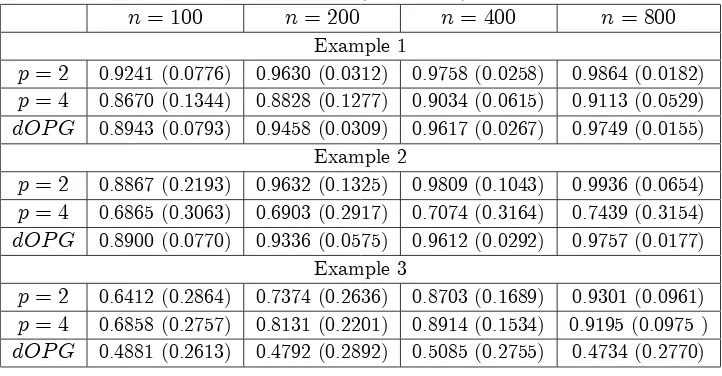
Table 2.1: Mean and Standard error (in brackets) of the inner productbT 0.
n= 100 n= 200 n= 400 n= 800
Example 1
p= 2 0.9241 (0.0776) 0.9630 (0.0312) 0.9758 (0.0258) 0.9864 (0.0182) p= 4 0.8670 (0.1344) 0.8828 (0.1277) 0.9034 (0.0615) 0.9113 (0.0529) dOP G 0.8943 (0.0793) 0.9458 (0.0309) 0.9617 (0.0267) 0.9749 (0.0155)
Example 2
p= 2 0.8867 (0.2193) 0.9632 (0.1325) 0.9809 (0.1043) 0.9936 (0.0654) p= 4 0.6865 (0.3063) 0.6903 (0.2917) 0.7074 (0.3164) 0.7439 (0.3154) dOP G 0.8900 (0.0770) 0.9336 (0.0575) 0.9612 (0.0292) 0.9757 (0.0177)
Example 3
p= 2 0.6412 (0.2864) 0.7374 (0.2636) 0.8703 (0.1689) 0.9301 (0.0961) p= 4 0.6858 (0.2757) 0.8131 (0.2201) 0.8914 (0.1534) 0.9195 (0.0975 ) dOP G 0.4881 (0.2613) 0.4792 (0.2892) 0.5085 (0.2755) 0.4734 (0.2770)
where g(u) = 12p1 +u2:. Here,
0;j = exp ( j)=qP4k=1exp ( 2k), j = 1; :::;4; and
the "t are as in the previous examples.All the three models can easily be veri…ed to be
geometrically ergodic by either Theorem 3.1 or Theorem 3.2 of An and Huang (1996),
and hence they are strictly stationary and strong-mixing with exponential decaying rates
(see Fan and Yao 2003, p. 70). In all examples, our goal was to estimate the optimal
orientation 0and the single-index predictive densityfYj Tx ytj Txt ofytgiven the lagged
observations xt = (yt 1; yt 2; yt 3; yt 4). For each model200 replications were generated
with sample sizes n= 100;200;400 and 800, and we implemented the method to produce
the corresponding estimatesband fe
YjbTX yjb T
x .
In practice, of-course, one does not know a priorily the optimal number of lagged
observations to be considered in the model, and the lag should be chosen according to
some preliminary analysis or model selection criterion. Cross-validatory techniques were
shown to have successful applications to model selection in semiparametric settings (Gao
and Tong 2004, Kong and Xia 2007), and they can be used to produce a stopping rule to
the single-index c.p.d.f. model. However, these computationally intensive techniques are
less desirable asbhas to found by numerical optimisation. The topic of model selection is thus left open for some further research, and a relevant discussion is given in the concluding
Table 2.1 presents the average and standard error (over 200 replications) of the inner
products bT 0 obtained for the three models with di¤erent sample sizes, and where the
estimation was performed using a kernels of orderp= 2,p= 4or by thedOP Gmethod of
Xia (2007). Since band 0 are both unit vectors, b
T
0 is simply jcos j, where is the
angle betweenband 0, and it is1 if and only ifb= 0. Note also that this inner product
is directly related to the sum of square error measure
b 0 2 = b 2+k 0k2 2 b T
0 = 2 1 b
T 0 :
As a general conclusion from Table 2.1, we can see that the orientation estimates become
more accurate as the sample size increases, although the rate of improvement is not as fast
as suggested by the theoretical asymptotic results. Comparing between the accuracy of the
orientation estimates across the three di¤erent models, one can see that the method seems
to be less accurate for the nonlinear models, and in particular for the nonlinear ARCH
model with relatively small sample sizes (n = 100 or 200). However, when the number
of observations is increased to800, the average of the inner product bT 0 is consistently
higher than 0:9 for all of the models with second-order kernels, and two out of the three
models with fourth-order kernels.
The generally better performances of the second-order kernels compared with the
fourth-order kernels in terms of the accuracy of the corresponding orientation estimates are
particularly striking in Examples 1 and 2. In Example 3, on the other hand, the
fourth-order kernel yields some more accurate estimates for 0 with sample sizesn= 100; 200or
400. However, when the sample size is increased to n = 800 the accuracy of the
second-order kernels ‘catches up’with that of the fourth-second-order kernels. An extensive investigation
performed by Marron and Wand (1992) of the e¤ectiveness of high-order kernels in
non-parametric density estimation provides an explanation for this discrepancy between theory
and practice as it shows that it may take extremely large sample sizes (with a typical order
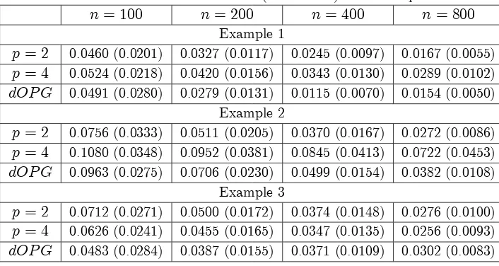
domi-Table 2.2: Mean and standard error (in brackets) of the sample RMSPE.
n= 100 n= 200 n= 400 n= 800
Example 1
p= 2 0.0460 (0.0201) 0.0327 (0.0117) 0.0245 (0.0097) 0.0167 (0.0055) p= 4 0.0524 (0.0218) 0.0420 (0.0156) 0.0343 (0.0130) 0.0289 (0.0102) dOP G 0.0491 (0.0280) 0.0279 (0.0131) 0.0115 (0.0070) 0.0154 (0.0050)
Example 2
p= 2 0.0756 (0.0333) 0.0511 (0.0205) 0.0370 (0.0167) 0.0272 (0.0086) p= 4 0.1080 (0.0348) 0.0952 (0.0381) 0.0845 (0.0413) 0.0722 (0.0453) dOP G 0.0963 (0.0275) 0.0706 (0.0230) 0.0499 (0.0154) 0.0382 (0.0108)
Example 3
p= 2 0.0712 (0.0271) 0.0500 (0.0172) 0.0374 (0.0148) 0.0276 (0.0100) p= 4 0.0626 (0.0241) 0.0455 (0.0165) 0.0347 (0.0135) 0.0256 (0.0093) dOP G 0.0483 (0.0284) 0.0387 (0.0155) 0.0371 (0.0109) 0.0302 (0.0083)
nant e¤ect to begin to be realised, and for the high-order kernels to produce more accurate
estimates. In particular, Marron and Wand (1992) conclude that high-order kernels are
not recommended in practice for kernels density estimation with realistic sample sizes.
The dOP G method seems to perform very well in Examples 1 and 2, although its
performance is inferior to that achieved with the second-order kernels. However, thedOP G
performs very poorly in Example 3, even for sample size n = 800, which suggests that
dOP Ghave di¢ culties in estimation of the optimal orientation where it is related to higher
moments ofX.
Notice that at the second-stage of estimation, fe
YjbTX yjb T
x is estimated using the
same second-order kernel. Thus, for the purpose of comparison between the approach
obtained with di¤erent implementation of the …rst-stage of estimation of the orientation
estimator,b, it is su¢ cient to examine directly the performance ofb. Nevertheless, for the sake of completeness and to illustrate the …nite-sample properties of the procedure, we now
continue and assess the accuracy of the conditional density estimator,fe
YjbTX yjb T
x . To
this end;we used the sample Root Mean Square Percentage Error (RMSPE),
RM SP E = n
P
i=1
h e
f
YjbTX yijb T
xi fYjX(yijxi)
i2 Pn i=1
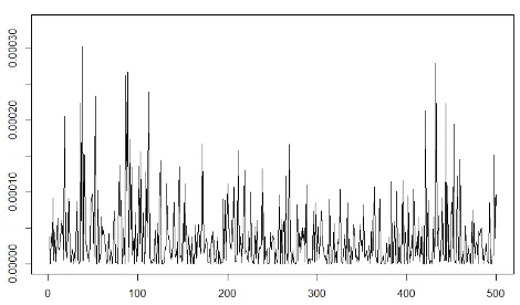
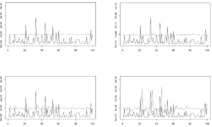
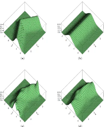
[image:34.612.144.497.118.306.2]Figure 2.1. Example 4: Daily exchange rate squared returns of the USD-GDP between 04/01/2010 and 30/12/2011.
wherefYjX(yijxi)is the real conditional density. The average and standard error (over200
replications) of the sample RMSPE are given in Table 2.2 for orientation estimates that
were obtained at the …rst stage of estimation using a kernels of order p= 2,p = 4 or by
thedOP G method of Xia (2007).
Here, we see that the estimation error given by the sample RMSPE consistently
de-creases as the sample size inde-creases for all the simulation settings. Observe that although
the average accuracy of the orientation estimates did not improve in Examples 1 and 2
betweenn= 200 and n= 400, the approximated conditional density obtained at the
sec-ond stage is more accurate on average for the larger sample size n = 400. Finally, as a
consequence of the orientation estimation performances, we see that in Examples 1 and 2
the conditional density estimates obtained by using second-order kernels (at the …rst-stage
of the estimation) outperforms the ones obtained with fourth-order kernels or withdOP G.
In Example 3, however, the estimates corresponding to fourth-order kernels are slightly
more accurate on average.
Example 4: Finally, we demonstrate a real-data application of the proposed method. In the standard ARCH(p) model, it is assumed that
where
t= 0+
Xp j=1 jy
2 t j:
Here, "t is a white noise process, 0 >0 and j 0; j = 1; :::; p. The ARCH(p) model
can be written as an AR(p) model in y2t, by the relation
yt2= 2t+ 2t "2t 1 = 0+
Xp j=1 jy
2
t j+"t;
where"t = 2
t "2t 1 is an heteroscedastic white noise process. This last formulation
mo-tivates us to consider an application of the proposed method to prediction of the volatility
process in terms of the squared returns (cf. Andersen and Bollerslev 1988). We use a
time-series of the daily exchange-rates’squared returns between the US Dollar (USD) and
the British Pound (GBP) between 4 January 2010 and 30 December 2011. The data
consists of 501 data points, out of which we allocate the last 100 points for prediction.
Figure 2.1 presents the time-series data over the full period. We implement the
approx-imation to estimate the predictive density fY2jTx yt2jxt of yt given the 4-lagged data
xt = y2t 1; y2t 2; y2t 3; yt2 4 . Using only the …rst 401 data points, we estimate …rst the
orientation vector, and the obtained estimate is b= (0:921;0:082;0:250; 0:288). This es-timate suggests that the most recent lag has the strongest e¤ect on the predictive density
of y2t, although the third and fourth lag also have some signi…cant e¤ect. Next, for any
observation yt that belongs to the last 100 observations, we iteratively construct a
predic-tive density model using the estimated orientation,b;where all nonparametric functional estimators rely on past information y21; :::; y2t 1 (that may include some past observations
from the last 100 data points). In order to examine the predictive capability of the models,
we construct the corresponding one-sided (1 ) prediction con…dence intervals, based
on the right tail of the density function, for the squared returns in the last 100 observations.
The reason we considered one-sided prediction intervals, rather than standard two-sided
ones, is that the density function of the squared returns is supported on [0;1), while
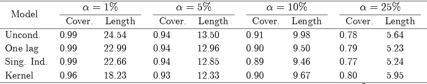
Model = 1%
Cover. Length
= 5%
Cover. Length
= 10%
Cover. Length
= 25%
Cover. Length
Uncond. 0.99 24.54 0.94 13.50 0.91 9.98 0.78 5.64
One lag 0.99 22.99 0.94 12.96 0.90 9.50 0.79 5.23
Sing. Ind. 0.99 22.66 0.94 12.85 0.89 9.46 0.77 5.24
[image:37.612.109.541.107.192.2]Kernel 0.96 18.23 0.93 12.33 0.90 9.67 0.80 5.95
Table 2.3: Results for Example 4: Prediction coverage (%) and avg. length (105) of
(1 ) prediction intervals.
completely capture the probability mass in the left tail of the volatility density. On the
other hand, the right tail of the volatility distribution is very heavy, and for practical
pur-poses, such as for risk management, the right tail of the volatility distribution seems to be
of much more interest than the left tail (see, for example, Windsor and Thyagaraja 2001).
Table 2.3 gives the prediction coverage (% of observationsy2t that fall inside the prediction
interval) and the average length of the prediction interval over the last 100 observations for
all obtained models with = 1%; 5%; 10%and 25%. For comparison, this table presents
the result obtained with the unconditional kernel density ofyt2 (Uncond.), the conditional
density based only on the most recent lag (One lag), the single-index approximation (Sing.
Ind.) and the standard multivariate kernel estimator (Kernel). Also, for visual
illustra-tion, Figure 2.1 shows plots of the last 100 observations and the corresponding right tail
90% prediction interval obtained by each model.
For all of the con…dence level values examined, the unconditional density estimator
pro-duced the widest prediction-intervals on average, while the standard unconditional density
estimator produced relatively narrow con…dence intervals. In terms of prediction coverage,
both the unconditional density estimator and the PPCDE provide relatively accurate
es-timates, while the standard conditional density kernel estimator has much less similar to
reality. We thus see that the PPCDE manages to provide increased accuracy and predictive
2.5 Appendix A - Proofs of the Theorems
Proof of Theorem 2.3.1. By assumptions (A4), (A6) it is su¢ cient (Amemiya 1985, Theorem 4.1.1) to prove that
sup
2 L
( ) ES logfYjTX yj Tx =op(1): (2.11)
DenoteL( )as the version ofL( )when conditional density estimates are replaced by the true conditional densities, that is,
L( ) =n 1
n
P
i=1
logfYj TX yij Txi :
By smoothness condition (A4) we have that for any" >0 there exists a positive constant
>0such that for any ( 1; y; x)2 S and 2U ( 1), a -ball with centre at 1,
logfYj TX yj Tx logfYj TX yj T1x < ":
As a result, we have
sup
2U( 1)
L( ) ES logfYjTX yj Tx
= 2"+ L( 1) ES logfYj TX yj T1x : (2.12)
Note also that since is compact, it is possible to construct a …nite open covering of by
-balls,U ( k) ,k= 1; :::; K. Thus, using (2.12) we have that for any" >0
P sup
2
L( ) ES logfYjTX yj Tx >3"
K max
k=1;:::;KP 2supU(
k)
L( ) ES logfYj TX yj Tx >3"
!
K max
k=1;:::;KP L( k) ES logfYj
The series logfYj TX yij Txi is itself strong-mixing (see, for instance, White 1984), and
by the ergodic theorem for strong-mixing processes (see Fan and Yao 2003, Proposition
2.8) we get for any 2
L( ) ES logfYj TX yj Tx !0 a:s:
We thus established that
sup
2
L( ) ES logfYj TX yj Tx =op(1): (2.13)
Next, by Lemma 2.6.5, all trimming-terms,bi,i= 1; :::; n, de…ned in (2.5), are
eventu-ally equal to 1 for any large enough n with probability 1. Therefore, we can consider
n to be large enough so we can ignore the trimming-terms, i.e. set bi 1. Since
fY; TX y; Tx ; f TX Tx are bounded from below by " > 0 on S and SX,
by the uniform consistency result of Lemma 2.6.2 and the continuous mapping theorem
(Amemiya 1985, Theorem 3.2.6) applied to the log-function we get withzj = (yj; xj),
sup
2 ;z2S
logfbY; TX y; Tx logfY; TX y; Tx = op(1);
sup
2 ;x2SX
logfbTX Tx logf TX Tx = op(1):
Therefore, we have
sup
2 jL
( ) L( )j
max
1 i nsup2 logfb i
Y; TX yi;
Tx
i logfY; TX yi; Txi
+ max
1 i nsup2 log
b
f TiX
Tx
i logf TX Txi
sup
2 ;z2S
logfbY; TX y; Tx logfY; TX y; Tx
+ sup
2 ;x2SX
logfbTX Tx logf TX Tx +o(1)
Results (2.13) and (2.14) imply (2.11), and therefore the Theorem is proved.
Proof of Theorem 2.3.2. As in the proof of Theorem 2.3.1, letL( )be a version of the likelihoodL( )when conditional density estimates are replaced by the true conditional densities,
L( ) =n 1
n
P
i=1
logfYj TX yij Txi :
Furthermore, lete= arg max 2 L( ). Note that by (2.13) in the proof of Theorem 2.3.1
and Theorem 4.1.1 of Amemiya (1985)eis a consistent estimator to 0.
Due to smoothness condition (A9), the mean value theorem, applied to the function
rL( ) with mean-value such that 0 e 0 ;yields
rL e rL( 0) =r2L e 0 : (2.15)
Since 0 lies in the interior of , the consistency ofe implies that for all" >0,
p
nrL e > " !p0: (2.16)
Moreover, By the central limit theorem (CLT) for -mixing processes (cf. Fan and Yao
2003, Theorem 2.21),
n1=2rL( 0)!dN(0; ( 0)): (2.17)
By smoothness condition (A9) and the ergodic theorem for strong-mixing processes (see
Fan and Yao 2003, Proposition 2.8), one can show by a similar way to (2.13), that
sup
2 r
2L( ) + ( ) =o
p(1): (2.18)
Note that by conditions (A6) and (A9) there is a generalised inverse of ( 0), denoted