http://dx.doi.org/10.4236/acs.2014.45080
Improved Retrieval of Sea Ice Thickness and
Density from Laser Altimeter
Vera Djepa
Department of Applied Mathematics and Theoretical Physics (DAMTP), Cambridge University, Cambridge, UK Email: [email protected]
Received 16 October 2014; revised 27 November 2014; accepted 10 December 2014
Copyright © 2014 by author and Scientific Research Publishing Inc.
This work is licensed under the Creative Commons Attribution International License (CC BY). http://creativecommons.org/licenses/by/4.0/
Abstract
RA. The results and algorithms, discussed in this paper are essential contribution to SIT and SID retrieval, satellite remote sensing, cryosphere, meteorology and improved weather and climate forecast.
Keywords
Sea Ice Thickness, Radar Altimeter, Laser Altimeter, Sea Ice Density, Freeboard, Arctic
1. Introduction
Sea ice plays an important role in the global climate system via feedbacks and ice-atmosphere heat exchange [1] [2]. The sea ice decline contributes to approximately one third of the observed increase in the central and north-ern European summer precipitation during 1979-2009 [3]. The ECHAM5 global atmospheric model simulations of the atmospheric response to decreased wintertime sea ice extend in the Barents and Kara seas shows that a small decrease in the ice concentration (from 100% to 80%) would result in an anomalous cyclonic circulation over the Arctic Ocean, whereas a larger decrease (from 80% to 40%) could result in an anticyclonic model pre-dicted circulation, associated with easterly winds over the surrounding continents, which may generate winter cooling of about −1.5˚C in large parts of Eurasia and North America [4]. Model simulations show that if the winter sea ice in the Barents and Kara Seas drops down to 1%, the circulation over the Arctic Ocean would turn to cyclonic again, generating winter warming over Eurasia and the USA. The model simulation confirm the high sensitivity of weather and climate forecast to accuracy of the SIT and the importance of a long term records of SIT distribution with corresponding uncertainties. The ice loss is linked to the sea ice albedo feedback and ra-diative greenhouse gas forcing. The ice thickness is essentially part of the lower boundary condition for Weather Research and Forecasting Model (WRF). Mesoscale simulations with the WRF have generally used a simple re-presentation for sea ice thickness and for snow depth on sea ice. For instance, the Noah land surface model ((LSM) for versions 3.4.1 and earlier of WRF) specify a sea ice thickness of 3 m. Because the ice thermodyna- mics and dynamic depend strongly on ice thicknesses the accuracy of the model forecast depends also on accu-racy of the SIT distribution.
Accurate SIT estimate is important for model validations and better understanding of the recent climate change. SIT distribution may help to answer the question: Is the ice thickness change part of a negative trend in the Arctic ice thickness, natural, inter-annual variability, model or algorithms parameterization.
Satellite laser altimeter (LA) (Ice, Cloud and land Elevation Satellite (ICESat)), Radar Altimetry (RA) (e.g. ERS1, 2, Envisat and CryoSat-2), airborne (Operational IceBridge (OIB)) and Upward Looking Sonar (ULS) on submarine, as well as the future (European Space Agency (ESA)/Sentinel and the National Aeronautics and Space Administration (NASA)/ICESat-2 missions with on board Advanced Topographic Laser Altimeter Sys-tem (ATLAS) (expected to be launched in 2015)) provide long term estimate of SIT and freeboard in the last three decades. The freeboard on snow/ice-air interface is extracted from LA by comparing the satellite distance from the snow or ice surface to that of ice free areas [5]. Using the equation for hydrostatic equilibrium the freeboard measurements from LA is converted to sea ice thickness, which is ice density (ρi), snow depth (hs),
density (ρs) and water density (ρw) depended as the SIT, retrieved from RA [6]. The SIT, which is available from
the National Snow and Ice Data Centre (NSIDC) is calculated from the freeboard, derived from ICESat, insert-ing constant densities for water, ρW = 1023.9 kg∙m−3, ice, ρi = 915.1 kg∙m−3 and snow, ρS (NSIDC, 2010).
Dif-ferent constant ice density (ρi = 925 kg∙m−3) has been inserted in the equation for hydrostatic equilibrium to
cal-culate SIT using the freeboard, which was derived from ICESat [10]. The SIT which is derived from the free-board, retrieved from LA (Airborne Topographic Mapper (ATM) on board OIB) is calculated by inserting in the equation of hydrostatic equilibrium fixed sea ice (ρi = 914.3 kg/m3), water (ρw = 1023.9 kg/m3) and snow (ρs =
264 kg/m3 during the expedition in 2009 and ρs = 320 kg/m3 during the expedition in 2010) densities, as well as
snow thickness derived from the snow radar on board OIB [5], which is different from the snow depth, which was used to retrieve SIT from ICESat [7]. The SIT has been retrieved from RA2/Envisat inserting in the equa-tion for hydrostatic equilibrium fixed ρi = 900 kg/m
3
[8] [9], hs and ρs from Warren Climatology (WC) [10]. The
(WC) over FYI and hs (WC) over MYI, requiring a-priory information for ice type [11]. Sensitivity analyses,
observations and laboratory study confirm the sensitivity of the retrieved SIT to potential errors associated with input variables (ρi, ρw,ρs, hs and the freeboard derived from LA and RA) when the equation for hydrostatic
equi-librium is applied [6] [12]. Using different input variables, with unknown accuracy in the equation for hydros-tatic equilibrium to convert the freeboard (which is derived from RA and LA) into SIT, is leading to not com-parative results of SIT and high biases of the derived SIT from different instruments [12]. Theoretical [13], ex-perimental [14], field [15] studies and sensitivity analyses [12] confirm the wide range of variability of sea ice density (from 720 kg/m3 to about 940 kg/m3) [16] and that the use of a constant ice density to retrieve SIT from the freeboard, derived from LA or RA will lead to not accurate estimate of SIT for the areas with different ice density due to ρi dependence on ice freeboard, thermodynamic properties and thickness of sea ice. The
sensitiv-ity analyses confirms that use of inaccurate ρi may lead to up to 2.7 m bias in the retrieved SIT for hfi = 0.27 m
in absence of snow depth [12]. The uncertainty analyses and validation studies confirm the increased accuracy of the derived SIT from RA if variable ice density (VID) is inserted in the equation of hydrostatic equilibrium to convert the freeboard into SIT [12]. Comparison of the collocated SIT derived from different instruments (RA/ERS-1/2, RA2/Envisat and ULS) show minimum biases when VID algorithm is applied and the same input parameters (ρw,ρs, and hs) are inserted in the equation for hydrostatic equilibrium to convert the freeboard into
SIT [12].
The purpose of this study is to develop and validate algorithm with corresponding error analysis to retrieve sea ice density and convert the freeboard (derived from LA) in SIT for climate applications, providing minimum bias with collocated SIT from independent satellite observations from RA. The paper is organized as follows: 1) The hydrostatic equations to convert the freeboard derived from RA and LA into SIT and the impact of contri-buting factors are discussed in Section 2; 2) Sensitivity, uncertainty analysis and retrieval of VID to derive SIT from LA are provided in Section 3; 3) Validation of the derived SIT from LA, using variable ice density and collocated SIT from RA is given in Section 4; 4) the final conclusions are provided in the last Section 5.
2. SIT Retrieval from the Freeboard Derived from Laser and Radar Altimeter
The SIT has been derived from the freeboard, retrieved from LA on board ICESat [7] [17], OIB/ATM [5] [17], or from RA on board ERS1, 2, Envisat and Cryosat-2 [8] [11], using the equation for hydrostatic equilibrium. Conversion of the freeboard, derived from LA and RA into SIT is freeboard, hs, ρs, ρi, ρw dependent and theac-curacy of the retrieved SIT depends on acac-curacy of the input variables.
The OIB mission has been developed to cover the gap between ICES at and ICESat2 for operational observa-tions of ice thickness in the Arctic and Antarctic and data from OIB are available from the NSIDC [17].The SIT is retrieved from the geo-located freeboard (hf) derived from the laser altimeter (ATM) on board OIB [17],
ap-plying the equation for hydrostatic equilibrium, which is snow depth, density, ice density and freeboard depen-dent, using constant ice density. The equation for hydrostatic equilibrium and the impact of input variables on retrieved SIT from the freeboard, derived from RA and LA are described in the next subsections.
2.1. Conversion of the Freeboard Derived from Laser Altimeter into Sea Ice Thickness
The SIT derived from laser altimeter (ATM) has been calculated by Equation for hydrostatic equilibrium, using different constant input variables for hs, ρi, ρs, ρw [5] [6]. Use of constant different snow densities (ρs = 264
kg/m3 during expedition in 2009 and ρs = 320 kg/m3 during expedition in 2010 [18], not accounting for snow
grain and roughness may lead to inaccurate snow depth retrieval in locations with different snow density and not precise estimation of hs and SIT from LA/ATM. The retrieved freeboard (hf) from LA is converted into sea ice
thickness, hi, applying the equation for hydrostatic equilibrium:
(
) (
) (
)
i w f w i w s s w i
h =
ρ
hρ
−ρ
−ρ
−ρ
hρ
−ρ
(1)where hs is the snow depth, ρi, ρs, ρw are the ice, snow and water densities [6]. Considering that the laser
altime-ter measures the freeboard on air snow inaltime-terface and accounting for Equation (1) the following relationship of the sea ice draft dla and surface elevation hf, measured from laser altimeter is obtained:
(
)
(
)
(
)
la s s i f i w i
d = h
ρ
−ρ
+ hρ
ρ
−ρ
(2)The ratio R of the sea ice draft and elevation is computed by:
(
)
(
)
(
)
(
)
la f s s i f w i i w i
R=d h = h
ρ
−ρ
hρ
−ρ
+ρ ρ
−ρ
(3)One can see that hi, dla and R depend on the same variables hshf, ρs, ρi, ρw and in absence of snow R depends
only on ice density (ice type). The ration R will be constant for the same ice type and absence of snow even if the elevation changes. Use of a constant ice density will lead to constant R for regions with hs = 0 m and
differ-ent ice types, which may lead to misleading assumption for the same ice type.
The SIT [17], which is derived from the freeboard retrieved from LA/ATM on board OIB (with uncertainty, σhfi < 0.03 m), applying the equation for hydrostatic equilibrium (Equation (1)) and constant ice density (ρi =
915.1 kg∙m−3 have been compared (for validation) with collocated SIT, which is retrieved from the freeboard, derived from RA2 on board Envisat (with the same uncertainties), using the Equation for hydrostatic equili-brium. In the next section is discussed the conversion of the freeboard, derived from RA into SIT.
2.2. Conversion of the Freeboard, Derived from Radar Altimeter into Sea Ice Thickness
Assuming hydrostatic equilibrium and that the radar returns are from snow-ice interface, the SIT, hi, derived
from RA is calculated as a function of snow depth (hs), density of water, ρw, ice, ρi, and snow, ρs by [6]:
(
)
(
)
i s s fi w w i
h = h
ρ
+hρ
ρ
−ρ
(4)The radar altimeter measures the freeboard on ice snow interface (hfi) in presence of dry snow and cold
condi-tions, The sea ice draft (SID) retrieved from RA, as a function of sea ice freeboard hfi, is calculated from the
dif-ference of SIT and the sea ice freeboard by:
(
)
(
)
ra i fi s s fi w w i
d = −h h = h
ρ
+hρ
ρ
−ρ
(5)where hi is calculated by Equation (4), assuming that the radar return is on snow-ice interface. One can see that
SIT, derived from RA depends on the same input variables and their uncertainties as the SIT derived from laser altimeter (snow depth and density, ice, water density and freeboard). Collocated sea ice draft, derived from RA (on board ERS and Envisat), with the sea ice draft, derived from ULS, in the Arctic has been used to validate the rithm for SIT retrieval, using the freeboard derived from RA to calculate SIT applying 6 algorithms and the algo-rithm with variable ice density was selected, providing minimum bias of the SID derived from RA and ULS [12]. The collocated SIT, retrieved from LA and RA using constant ρi and variable ρi will be validated in Section 4.
The impact of the input variables (hs, ρs, ρi, ρw and hfi) on the retrieved SIT, applying the equation for hydrostatic
equilibrium will be discussed in the next sub-sections.
2.3. Impact of Sea Ice and Water Density on Retrieved SIT from LA
The sea water density, ρw, depends on salinity, S, temperature, T, and pressure and ranges from about 1022
kg/m3 at the sea surface to 1050 kg/m3 at the bottom of the ocean. The density of sea water across the Beaufort Shelf and slope off Alaska varies between 1023.2 kg/m3 in October to 1024.2 kg/m3 in April and a mean value of ρw = 1024 kg/m
3
has been used for SIT retrieval from ICES at [7]. Water density ρw = 1025 ± 0.5 kg/m
3
has been used to calculate mean MYI sea ice density (882 kg/m3) [16].
The density of sea ice depends on density of pure ice, the fractional volume of air pockets and the sea ice freeboard [16]. The density of pure ice at 0˚C is 916.4 kg∙m−3 and is increasing to 919.3 kg/m3 at −30˚C [19]. The density of sea ice can be greater than these values because of the effect of brine inclusions in the ice, or less because of the effect of air bubbles, temperature and ice type. Sea ice densities below the waterline have typical values between 920 and 940 kg∙m−3[16].
Sea ice density has been calculated from different authors as a function of hfi, hs and ρs, using the equation for
isostatic equilibrium, or field observations [15] [16]. The MYI ρi can vary between 720 and 900 kg∙m−3 and the
ice density depends on temperature, free-board, snow depth, or melting [16]. The typical FYI ρi is in the range
910 - 920 kg∙m−3[19]. Mean MY ice density 882 ± 23 kg/m3 is calculated by [16], which is less than ρi = 914.3
[15], experimental studies [14] and sensitivity analyses confirm dependence of ρi on ice type, thermodynamic
properties and hfi. A linear relationship has been obtained between ρi and “effective” ice free-board, hfie (m),
which depends on sea ice freeboard, hfi, snow depth, hs, density, ρs and the mean MY ice density [15]. By
com-parison with in-situ (drilling) observations, it was concluded that a VID model provides more accurate results for freeboard to SID conversion using the equation for hydrostatic equilibrium, compared with fixed sea ice density, used to convert the freeboard into sea ice draft. The following regression of sea ice density, ρiKO, on SIT
has been derived based on laboratory study, confirming the ρi dependence on hi[14]:
0.5 iKO 0.9363 0.0018hi
ρ
= − (6)Observations [15] [16] and laboratory study [14] confirm the wide range of sea ice density variations and ρi
dependence on hfi, hi, hs and ρs. Variable ice density algorithm (described in Section 2.5), inserted in the
equa-tion for hydrostatic equilibrium (Equaequa-tion (1)) has been validated with the field [15], laboratory study [14] and collocated SIT, derived from RA (Section 4). The impact of snow depth on retrieved SIT from LA is discussed in the next subsection.
2.4. Impact of Snow Depth on Retrieved Sea Ice Thickness from Laser Altimeter
Snow depth is an input variable to retrieve SIT from LA, using the hydrostatic equation (Equation (1)). Snow is a dielectric structure consisting of air, ice particles and liquid water. The dielectric constant of snow is a function of frequency, temperature, volumetric water content, snow density, shape of ice particles and water inclusion. Wet snow is a mixture of ice crystals, liquid water and air, and the dielectric constant of snow over sea ice de-pends on salinity. The density of wet snow can be approximated as a function of density of dry snow and volu-metric water content (W). The snow, that is older than one year (over MYI) is a mixture of ice and water par-ticles with different grain size and particle volume content and may becomes glacier ice, leading to ice scattering on effective freeboard within the snow layer. Presence of ice particles, ice lenses or frozen snow pack lead also to ice density contribution within the snow pack. Observations and model simulations confirm internal ice layers and presence of an effective ice freeboard within the snow pack, depending on hfi, hs and ρs. Models demonstrate
that the snow density changes due to melt frees metamorphism and when the water freezes the snow density in-creases [13]. Snow crusts that occur after refreezing of melted snow can achieve densities of 700 - 800 kg∙m−3. The older than one year snow is a mixture of ice and water particles with different grain size and particle volume content and may become glacier ice at a density of about 830 kg∙m−3, which is leading to radar signal scattering within the snow layer. Thus, the radar scattering surface depends on hs, ρs and hfi and is equal to hfi if there is no
snow on the ice surface or in presence of dry snow. The ice freeboard for laser altimeter could be within the snow layer in presence of frozen snow, or snow crusts that occur after refreezing of melted snow. Snow depth derived from WC, AMSRE, OIB snow radar, or models have been inserted in Equation (1) from different au-thors to retrieve SIT from LA, which lead to different results [5] [6]. The snow depth and density from WC are validated over about 40 years in the Arctic and are available with corresponding uncertainties as a function of latitude, longitude and mean monthly snow depth [10]. WC has been used successfully until now for low resolu-tion (100 km spatial and 1 month temporal resoluresolu-tion) SIT retrieval from RA, ICESat and CryoSat-2 with cli-mate applications [7]-[9] [11]. Recent limited high resolution observations of snow depth from buoy, OIB/snow radar and microwave radiometer (AMSR-E) suggested decreased snow depth over First Year Ice (FYI) with not proofed accuracy [18] [20] [21]. AMSR-E snow depth retrieval algorithm, ECMWF re-analyses and surface ob-servations [21] confirm underestimation of the observed snow depth from AMSR-E satellite observations. The snow depth, retrievals from the OIB snow radar, depends on accuracy of estimated air-snow and snow-ice inter-faces [5] and the distance between the two interfaces, which is a function of snow and air dielectric constants and snow density. Very low constant snow density (264 kg/m3) has been used to retrieve snow depth in April 2009 [18]. The mean snow density from WC for this month is ρs = 320 kg/m3[10] and for FYI the ρs = 324
re-trieved snow depth from the OIB snow radar depends on the accuracy of estimated snow-air interface, ice-snow interface and snow density. Thus, using constant snow density, not accounting for snow grain and roughness, and considering the strong dependence of the algorithm on snow-ice and snow-air freeboards, may lead to inac-curate snow depth retrieval from OIB/radar in locations with different snow density or not precise estimation of hfi or hfs. According to [5] there were not validation data for snow depth, retrieved from OIB/radar in 2010 and
the algorithm was changed, which makes questionable the accuracy of the retrieved snow depth from OIB/snow radar. Collocated hs (from WC and OIB snow radar), freeboard (hf) (derived from ATM/OIB with uncertainty σhf
< 0.03 m), averaged in 100 km spatial resolution and centered in the hfi averaged area (derived from RA with
ra-dius 100 km and uncertainty σhfi < 0.03 m) have been used to calibrate the snow depth retrieval from the OIB
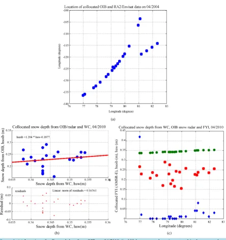
snow radar and examine the hs impact on accuracy of the retrieved SIT. The statistic is provided in Table 1 and
the area of observations, function of latitude (la) and longitude (lo) is shown on Figure 1(a).
(a)
[image:6.595.90.535.218.690.2](b) (c)
Figure 1. (a) Location of collocated data from OIB, on 04/2010 (in 100 km averaged area), centered in the averaged area (with 100 km radius) of the freeboard, retrieved from RA2/Envisat; (b) Collocated snow depth from OIB/radar and WC; (c) Collocated hs (WC) m, hs (OIB) m (red) and FYI (
*
Table 1. Statistic of collocated snow depth, freeboard and FYI, derived from OIB and RA2/Envisat.
Variable hf (m) OIB hfi (m) RA hfiw (m) OIB hfib (m) OIB hsw (m) WC hsoib (m) OIB FYI (%) ρs (WC) kg/m3 σhf (m)
Mean 0.542 0.1904 0.1964 0.314 0.345 0.228 3.27 303.9 0.0175
Std 0.0843 0.0626 0.0825 0.0918 0.005 0.0362 8.87 3.1 0.0057
One can see that the sea ice freeboard (hfib), estimated as a difference of the freeboard, hf, derived from
ATM/OIB and the snow depth, retrieved from OIB snow radar hsoib is with 0.224 m higher than the ice freeboard,
hfi, derived from RA2. The bias of hfiw (hfiw = hf− hsw(WC), where hsw is the collocated snow depth from WC)
and hfi is only 6mm, when, snow depth from WC is applied. The statistic (Table 1) and the regression of the
snow depth (Figure 1(b)) derived from OIB radar and the hsw(WC) confirm that OIB radar underestimate the
snow depth with 12 cm in comparison with hsw(WC):
( )
1.204 0.1877 m
soib sw
h = h − (7)
The underestimated snow depth, derived from OIB/radar cannot be explained with presence of FYI because it is only 3.2% presence of FYI in the area (Table 1), estimated from the collocated AMSR-E data. One can see that it is not any correlation (r = 0.273) between the hsoib and presence of FYI (Figure 1(c)), which confirms that
the lower hsoib values measured by OIB/snow radar are due to algorithm restrictions, but do not depend on
pres-ence of FYI. The mean snow density from WC for the observed area is ρs = 303.9 kg/m
3
(Table 1) and using a different constant snow density (ρi = 320 kg/m
3
) [5] to derive snow depth from OIB/snow radar is introducing error in the retrieved snow depth, which will impact the accuracy of the SIT derived from ATM/OIB. Use of a very low snow depth, constant snow and ice density (ρi = 914.3 kg/m
3
) [5], corresponding to FYI, in presence of MYI, will lead to over estimated SIT, derived from ATM/OIB, confirmed with statistic (Section 4). Statistics (Table 1) confirm the applicability of WC (hsw) to retrieve low resolution SIT from ATM/OIB (with climate
ap-plications), providing only 6 mm bias with the ice freeboard derived from RA, compared with 22.4 cm bias when snow depth from OIB/radar has been used. Equation (7) can be applied to improve and calibrate the algo-rithm for low resolution snow depth retrieval from OIB/snow radar. Retrieval of effective freeboard and the al-gorithm for VID, using hsw and ρs from WC is discussed in the next subsection.
2.5. Algorithm for Variable Ice Density
Using the equation for hydrostatic equilibrium (Equation (1)), ρi has been calculated for a wide range of input
variables hfi (from 0.09 m to 0.45 m), ρs(from 260 kg/m
3
to 360 kg/m3), hs (from 0.01 m to 0.38 m) andρw =
1024 kg/m3. The simulated ρi have been compared with the ρi derived from field observations [15] and
labora-tory study [14] and a linear dependence of a VID (ρiVID) and an effective freeboard (hfie) has been retrieved.
Re-gression coefficients have been derived satisfying the best fit of simulated ρiVID with that derived from the field
and laboratory study:
iVID ahfie b
ρ
= + (8)where a = −95.05, b = 930.4, mean ice density for FYI (ρiFYmean = 910 kg/m3) and hfie < 0.18 m;
a = −214, b = 948, mean ice density for MYI (ρiMYmean = 882 kg/m3) and 0.18 m < hfie < 0.37 m;
a = −36.54, b = 903.7, mean ice density for MYI (ρiMYmean = 882 kg/m3) and hfie > 0.37 m.
The mean ice density of MYI (ρiMYmean = 882 kg/m3), retrieved by [16] and ρiFYmean (ρiFYmean = 910 kg/m3) for
FYI, estimated based on laboratory study [14] have been inserted in Equation (9) to calculate the effective scat-tering surface (hfie), which is approximated as a function of hfi, hs, ρs and the mean MY and FY ice density,
ρimean:
(
mean)
fie f s s s i fiw
h =h − +h h
ρ ρ
=h +C (9)where hs and ρs, calculated as a function of latitude and longitude from WC and collocated with the freeboard,
derived from LA are inserted in Equation (9). The sea ice freeboard for cold and dry conditions, hfiw, is
calcu-lated as a difference of the hf, derived from LA/OIB and hs(WC) and the effective scattering surface, hfie is equal
to hfiw if it is not snow on the ice surface. The effective scattering layer within the snow pack depends on hs, ρs
m, ρsmax(WC) = 325 kg∙m3 and ρimean = 910 kg/m3, and Cmax(MIY) = 0.1327 m for ρimean = 882 kg/m3. The un-
certainty of the retrieved variable ice density (ρiVID) depends on uncertainties of the sea ice freeboard, hfi. For
example, the uncertainty of the VID is σρiMYVID = ±3.45 kg/m3 for MYI and σρiFYVID = ±2.85 kg/m3 for FYI and
the sea ice freeboard uncertainty (σhfi ± 0.03 m), where σρiVID will decrease if the accuracy of hfi increases. The
impact of the ice density and snow properties on accuracy of the retrieved SIT from LA and RA, using the equa- tion for hydrostatic equilibrium, is estimated by sensitivity and uncertainty analyses.
3. Sensitivity and Uncertainty Analyses of the Retrieved Sea Ice Thickness from
Laser and Radar Altimeter
Sensitivity analysis is applied to estimate sensitivity of the retrieved SIT from LA to input variables. Uncertainty analysis is applied to estimate the error of the retrieved SIT from LA, applying the equation for hydrostatic equi- librium.
3.1. Sensitivity of the Retrieved Sea Ice Thickness from Radar and Laser Altimeter
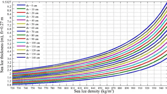
The sensitivity of SIT to input variables (ρi, hs and hfi) is analyzed (applying the equation for hydrostatic
equili-brium) where SIT is calculated for ρi = 720 - 950 kg/m3, hfi = 0.09 - 0.45 m, hs = 0 - 140 cm, ρs from WC and ρw
= 1024 kg/m3 (seeFigure 2).
The sensitivity analyses (Figure 2) shows that the impact of ice density on retrieved SIT is essential and the snow depth impact increases when hs increases. The impact of change of snow depth (from 0 to 140 cm) and ice
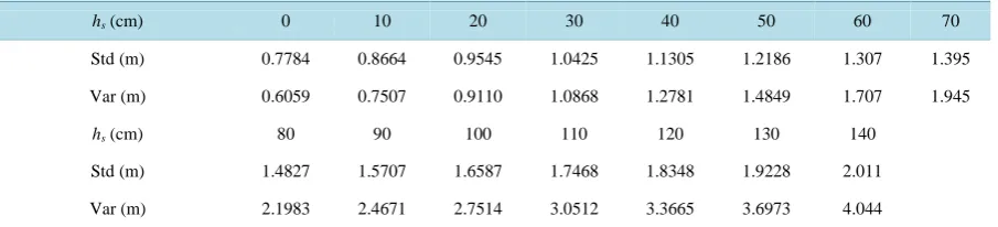
density (from 720 to 950 kg/m3) on standard deviations of the derived SIT, using the equation for hydrostatic equilibrium is shown in Table 2.
For snow depth 30 cm, the standard deviation of retrieved SIT due to impact of ice density is up to 1.04 m. The impact of ice density on uncertainties of the retrieved SIT is 0.78 m in presence of bare ice and increases with only 9 cm if the hs increases with 10 cm, which confirms higher impact of ice density variations on
uncer-tainties of the derived SIT, compared with the hs impact. The sensitivity analyses confirms that the ice density is
the most important variable that impacts the accuracy of the SIT retrieved from LA and use of inaccurate ρi may
lead to up to 2.7 m bias in the retrieved SIT for hfi = 0.27 m in absence of snow depth and ice density range (720
kg/m3 < ρi < 950 kg/m3) (Figure 2). Only a variable freeboard-dependent ice density, which considers the ice
type and snow depth along the RA track, will minimize the impact of uncertainties in the retrieved SIT from LA by inserting VID in Equation (1). The sensitivity analysis confirms that the ice density is the most important va-riable, which impacts the accuracy of the retrieved SIT from RA. The uncertainty of the derived SIT is up to 0.778 m due to ρi impact (for hfi = 0.01 m and hs = 0 m) and increase of the snow depth with 10 cm lead to
in-crease of the standard deviation with only 9 cm when the equation for hydrostatic equilibrium is applied. Use of a wrong fixed ice density could introduce up to 3.6 m bias of the retrieved SIT for hs = 30 cm (Figure 2). The
uncertainties of the retrieved SIT from LA, inserting variable ice density, hs and ρs from WC in the equation for
[image:8.595.175.449.540.694.2]hydrostatic equilibrium is discussed in the next section.
Table 2. Standard deviation of SIT for snow depth from 0 to 140 cm and ice density from 720 to 950 kg/m3.
hs(cm) 0 10 20 30 40 50 60 70
Std (m) 0.7784 0.8664 0.9545 1.0425 1.1305 1.2186 1.307 1.395
Var (m) 0.6059 0.7507 0.9110 1.0868 1.2781 1.4849 1.707 1.945
hs(cm) 80 90 100 110 120 130 140
Std (m) 1.4827 1.5707 1.6587 1.7468 1.8348 1.9228 2.011
Var (m) 2.1983 2.4671 2.7514 3.0512 3.3665 3.6973 4.044
3.2. Uncertainty Analysis of the Retrieved SIT from LA
Only the uncertainties, associated with conversion of freeboard to thickness (using the equation for hydrostatic equilibrium) will be analyzed. Assuming that the input variables in Equation (1) are uncorrelated, the uncertain-ty (εhi) of the retrieved thickness, hi, from the freeboard, measured from LA, will depend on propagated
uncer-tainties of the input variables:
i
h him p
ε
=ε
(10)where him is the mean ice thickness and the propagated uncertainty εp is calculated from the standard deviations
(σhf and σhs, σρs,σρw,σρi) of the freeboard, hf, snow depth, hs, snow, ρs, water, ρw, and ice, ρi, densities and
corres-ponding mean values of all contributing factors (mean freeboard (hfm), water, ice and snow densities, ρwm, ρim,
ρsm and snow depth, hsm):
(
)
(
) (
) (
)
(
) (
) (
) (
)
(
)
2 2 2
2
2 2 2 2 2
.
w w i
w w s i
p hf fm wm wm im
wm wm sm im hs sm
h
h
ρ ρ ρ
ρ ρ ρ ρ
ε σ σ ρ σ ρ σ ρ
σ ρ σ ρ σ ρ σ ρ σ
= + + +
+ + + + +
(11)
The mean ice density (him), propagated εp and total uncertainty, εhi, are calculated for the mean and standard
deviations of the contributing factors of SIT derived from OIB (Table 1)) (inserting snow depth from OIB radar and constant snow (ρsm = 320 kg/m3) and ice density (including hfm = 0.542 m, hsm = 0.2281 m, ρsm = 320 kg/m3,
ρwm = 1024 kg/m
3
, ρi = 314.3 kg/m
3
and corresponding standard deviations: σhf = 0.0175 m and σhs = 0.0362 m,
σρs = 19.2 kg/m3 and σρi = 25.15 kg/m3) and compared with εhi when variable ice density is inserted in Equation
(1) (using mean snow density and depth according to WC (ρsw = 303.9 kg/m3 with σρsw = 3.1 kg/m3, hsw = 0.345
m, σhsw = 0.005 m), ρimean = 892.2 kg/m3 and σρi = 3.05 kg/ m3 (see Table 4). The impact of fixed ice density
(and snow depth from OIB/radar) and variable ice density (snow depth and density from WC) on accuracy of the retrieved SIT from LA is demonstrated with Table 3.
One can see from Table 3 that the uncertainty of the derived SIT applying variable ice density is decreased 7.6 times compared with the εεhi estimated for hs derived from OIB radar, fixed ρs and ρi. The uncertainty εhi will
further decrease when a variable ice density is applied if the accuracy of the freeboard retrieval is increased. The propagated uncertainties of the retrieved SIT decrease (from 17.5% to 3%, Table 3) when VID (ρiVID) is inserted
in the equation of hydrostatic equilibrium. The algorithm to retrieve SIT from LA using variable ice density has been validated using collocated SIT derived from RA2 on board Envisat.
4. Validation of Sea Ice Thickness Derived from Laser Altimeter with Collocated
Sea Ice Thickness Retrieved from Radar Altimeter
A data base (Round Robin Data Package (RRDP)) of collocated SID and SIT from RA, OIB data, ULS and snow depth and density from WC have been developed as part of the European Space Agency (ESA) Climate Change Initiative (CCI) sea ice Essential Climate Variable (ECV) project (SICCI, 2013) [9]. The database in-cludes the following collocated data sets: 1) snow depth and density from WC with the same spatial resolution, time and location as the averaged freeboard derived from RA data; 2) submarine ULS SID data averaged over 50 km and collocated with hfi, derived from RA; 3) collocated snow depth, freeboard and SIT from NSIDC/OIB
Table 3. Impact of fixed ice density (OIB) and VID on uncertainty of the derived SIT.
Alg. OIB
him (hs(OIB))
OIB
ρ
ε (hs(OIB))
OIB
εhi (hs(OIB))
VID
him (hs(WC))
VID
ρ
ε (hs(WC))
VID
εhi (hs(WC))
m 3.379 0.175 0.591 2.31 0.0369 0.0776
Table 4. Statistics of the SIT derived from collocated freeboard, retrieved from laser and radar altimeter.
Variable SIT (LA, VID, hs(WC)) SIT (RA, VID, hs(WC)) SIT (RA, fixed ρi, hs(WC)) SIT (fixed ρi, hs(OIB)) ρi (kg∙m−3)
Mean (m) 2.125 2.124 2.275 3.379 892.2
Std (m) 0.445 0.358 0.455 0.750 3.053
B (m) 0 −0.001 −1.1 0 na
freeboard, derived from RA and RA2, averaged within an area of 100 km radius centered at each transect center. The sea ice freeboard is derived from ERS1, 2/RA and Envisat/RA2 data using the methodology described in [9]. The VID algorithm has been validated with collocated SID from ULS and SID derived from RA (ERS1, 2 and Envsat) within 12 years in the Arctic and has been selected for SIT retrieval from the freeboard derived from radar altimeter based on statistics (minimum bias and RMSE) [12]. The freeboard derived (with uncertain-ties σhf < 0.03 m) from NSIDC/OIB/LA/ATM, averaged in 100 km and centered in the averaged collocated
freeboard, derived from RA2 (Envisat), hs and ρs (from WC), OIB snow radar and presence of FYI from
AMSR-E have been used for validation of the VID algorithm to retrieve SIT from LA. The collocated SIT (OIB/LA), calculated by Equation (1) (for fixed sea ice density of 914.3 kg/m3, ρw = 1023.9 kg/m3, snow ρs =
320 kg/m3 and snow depth from OIB radar [5]) with SIT, derived from RA2 (calculated by (Equation (4), (algo-rithm A1, applied to retrieve SIT from Envisat and ERS1, 2, using fixed ρi = 900 kg/ m3, ρw = 1030 kg/m3, ρs
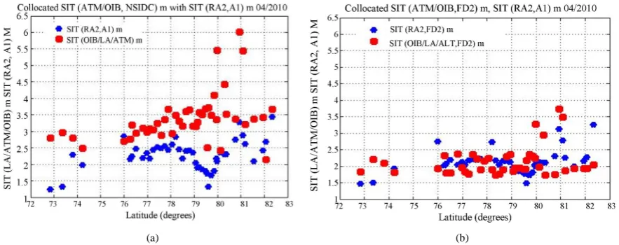
and hs from WC) are compared and shown on Figure 3(a). The statistics are summarized in Table 4. Due to use
of different input variables (ρw, ρs, ρi and hs) to calculate SIT from laser and radar altimeter the mean bias is up
to −1.1 m (Table 4), which makes impossible use of SIT derived from LA/OIB for comparison and validation of low resolution SIT, retrieved from RA.
The collocated SIT, derived from laser and radar altimeter, applying VID algorithm, inserting (in Equation (1) and Equation (4)) and the same freeboard (used to calculate SIT on Figure 3(a)) are compared on Figure 3(b) and the statistics is given in Table 4. The bias is estimated as: B = mean (hi(OIB)-hi(RA2)). One can see that the
mean bias of SIT derived from RA2 and LA/OIB has been reduced (from BB = −1.1 m) (for SIT calculated by RA2(A1) and LA(NSIDC/OIB), using different fixed ice densities and snow depth from OIB/radar) to B = 0.001m when variable ice density (VID algorithm) has been applied to calculate SIT from LA and RA and the same snow depth. Figure 3 and Table 4 confirm the applicability of ATM/LA/OIB for validation of low resolu- tion SIT, derived from RA, if the algorithm for variable ice density is inserted in Equation (1), using the same ρs
and hs to retrieve SIT from LA and RA. The improved bias of the SIT derived by LA/OIB and RA2 when VID
algorithm is applied confirms the higher accuracy and reduced biases of derived SIT from RA and LA when a variable ice density is inserted in the equation for hydrostatic equilibrium to transform the measured freeboard from LA into SIT. The VID algorithm, integrated with hs and ρs from WC, to retrieve SIT from ATM/OIB pro-
vides a new product of low resolution SIT from OIB/ATM, applicable for validation of SIT, derived from satel- lite RA for climate application. The VID algorithm provides also a sea ice density distribution, calculated from the freeboard, derived from ATM/OIB, which is important essential climate variable (ECV) for improved ice and climate model forecast. Statistic of the variable ice density (Table 4), calculated as a function of the meas-ured snow freeboard from ATM/OIB, snow depth and density from WC, is given in Table 4. The following re-gression equations have been retrieved confirming the ice density dependence on hi and hf:
5.3446 904.56, with RMSE 0.1574
i hi
ρ = − + = (12)
36.17 911.8, with RMSE 0.1659
i hf
ρ
= − + = (13)where hi and hf are the SIT and freeboard derived from LA/ATM/OIB, using variable ice density.
Using the regression Equations (12)-(13), ρi can be derived as a function of the measured freeboard from LA
(a) (b)
Figure 3. (a) SIT (OIB/LA, NSIDC) m (red), collocated with SIT (RA, A1) m (blue); (b) SIT (OIB/LA, VID) collocated with SIT (RA, VID).
tions (12)-(13) may have wide application for improved snow, ice, weather and climate forecast.
5. Conclusions
This paper has been focused on improved SIT and ice density retrieval from LA for climate applications. The main outcomes are:
1) Improved algorithm is developed and validated to convert the freeboard, derived from LA into SIT, using the equation for hydrostatic equilibrium and variable ice density. The algorithm has been applied to retrieve SIT from LA/OIB and validated with SIT derived from laboratory, field and satellite observations.
2) The impact of ice density and snow depth on accuracy of the retrieved SIT from LA is examined applying sensitivity analyses and equation for hydrostatic equilibrium. The sensitivity analyses confirms the high im-pact of ice density on accuracy of the derived SIT from LA (σhi = 0.778 m due to ρi impact, for hfi = 0.01 m
and hs = 0 m) and increase of the snow depth with 10 cm lead to only 9 cm increase of the σhi when the equa-
tion for hydrostatic equilibrium is applied. Use of a wrong fixed ice density could introduce up to 3.6 m bias of the retrieved SIT for hs = 30 cm.
3) The impact of hs, hf and ρs on accuracy of the retrieved SIT from LA, is analyzed and compared, applying
uncertainty analyses, inserting variable and fixed ice density in the equation for hydrostatic equilibrium. The uncertainty of the derived SIT applying variable ice density decreased 7.6 times compared with the εhi
esti-mated for hs derived from OIB radar, fixed ρs and ρi.
4) The algorithm for variable ice density is validated by comparison of collocated SIT, derived from ATM/OIB, with SIT, retrieved from RA2 and the bias is reduced from 1.1 m to 1 mm when variable ice density is in-serted in the equation for hydrostatic equilibrium, which confirms the accuracy of the developed VID algo-rithm and its applicability to create a long term time series of low resolution SIT, derived from LA and RA. 5) A new product of variable ρi, derived from LA/ATM/OIB is retrieved and regression equations are extracted
confirming ρi dependence on hi and hf. Until now fixed ice density has been assumed for SIT retrieval and
forecast. Extracting a variable ice density from the freeboard derived from LA/OIB is essential contribution for sea ice model validation, weather and climate forecast.
The developed algorithm to convert the freeboard, derived from LA in SIT, using variable ice density is es- sential contribution to ESA, NASA, NSIDC and climate programs, providing long term time series of SIT and ice density for climate and forecast models.
Acknowledgements
References
[1] Cheng, B., Mäkynen, M., Similä, M., Rontu, L. and Vihma, T. (2013) Modelling Snow and Ice Thickness in the Coas- tal Kara Sea, Russian Arctic. Annals of Glaciology, 54, 105-113. http://dx.doi.org/10.3189/2013AoG62A180
[2] Stroeve, J., Holland, M.M., Meier, W., Scambos, T. and Serreze, M. (2007) Arctic Sea Ice Decline: Faster than Fore-cast. Geophysical Research Letters, 34, Article ID: L09501. http://dx.doi.org/10.1029/2007GL029703
[3] Screen, J.A. and Simmonds, I. (2013) Exploring Links between Arctic Amplification and Mid-Latitude Weather. Geo-physical Research Letters, 40, 959-964. http://dx.doi.org/10.1002/grl.50174
[4] Petoukhov, V. and Semenov, V.A. (2010) A Link between Reduced Barents-Kara Sea Ice and Cold Winter Extremes
over Northern Continents. Journal of Geophysical Research, 115, Article ID: D21111.
http://dx.doi.org/10.1029/2009JD013568
[5] Kurtz, N.T., Farrell, S.L., Studinger, M., Galin, N., Harbeck, J., Lindsay, R., Onana, V., Panzer, B. and Sonntag, J.G. (2012) Sea Ice Thickness, Freeboard, and Snow Depth Products from Operation Ice Bridge Airborne Data. Cryosphere Discussions, 6, 4771-4827. http://dx.doi.org/10.5194/tcd-6-4771-2012
[6] Kwok, R. (2010) Satellite Remote Sensing of Sea Ice Thickness and Kinematics a Review. Journal of Glaciology, 56, 1129-1140. http://dx.doi.org/10.3189/002214311796406167
[7] Kwok, R., Cunningham, G.F., Wensnahan, M., Rigor, I. and Zwally, H.J. (2008) Thinning and Volume Loss of the Arctic Ocean Sea Ice Cover: 2003-2008. Journal of Geophysical Research, 114, Article ID: C07005.
http://dx.doi.org/10.1029/2009JC005312
[8] Connor, L., Seymour, W., Laxon, B., Ridout, A.L., Krabill, W.B. and McAdoo, D.C. (2009) Comparison of Envisat Radar and Airborne Laser Altimeter Measurements over Arctic Sea Ice. Remote Sensing of Environment, 113, 563-570.
http://dx.doi.org/10.1016/j.rse.2008.10.015
[9] (2013) Algorithm Theoretical Basis Document SICCI-ATBD.
http://icdc.zmaw.de/fileadmin/user_upload/ESA_Sea-Ice-ECV/SICCI_ATBDv1_D2.6_Issue1.1.pdf
[10] Warren, S. and Rigor, I. (1999) Snow Depth on Arctic Sea Ice. Journal of Climate, 12, 1814-1829.
[11] Laxon, S., Giles, K.A., Ridout, A.L., Wingham, D.J., Willatt, R., Cullen, R., Kwok, R., Schweiger, A., Zhang, J., Haas, C., Hendricks, S., Krishfield, R., Kurtz, N., Farrell, S. and Davidson, M. (2013) CryoSat-2 Estimates of Arctic Sea Ice Thickness and Volume. Geophysical Research Letters, 40, 1-6. http://dx.doi.org/10.1002/grl.50193
[12] Djepa, V. (2014) Sensitivity Analyses of Sea Ice Thickness Retrieval from Radar Altimeter. Journal of Surveying and Mapping Engineering (JSME), 2, 44-55.
[13] Hallikainen, M. (1992) Review of the Microwave Dielectric and Extinction Properties of Sea Ice and Snow. Geos-ciences and Remote Sensing Symposium, IGARSS 92, 2, 961-965.
[14] Kovacs, A. (1996) Sea Ice. Estimating the Full Scale Tensile, Flexural and Compressive Strength. CRREL (Cold Re-gions Research and Engineering Laboratory) Report 96-11, Hanover, New Hampshire 03755-1290, USA.
[15] Ackley, S.F., Hibler III, W.D., Kugzruk, F., Kovacs, A. and Weeks, W.F. (1976) Thickness and Roughness Variations of Arctic Multiyear Sea Ice. CRREL (Cold Regions Research and Engineering Laboratory) Report 76-18, 24 p, Hano-ver, New Hampshire 03755-1290, USA.
[16] Alexandrov, V., Sandven, S., Wahlin, J. and Johannessen, O.M. (2010) The Relation between Sea Ice Thickness and Freeboard in the Arctic. The Cryosphere Discussion, 4, 373-380. http://dx.doi.org/10.5194/tc-4-373-2010
[17] NSIDC (National Snow and Ice Data Centre) (2014). http://nsidc.org/data/icebridge/
[18] Farrell, S.L., Kurtz, N.T., Connor, L., Elder, B., Leuschen, C., Markus, T., McAdoo, D.C., Panzer, B., Richter-Menge, J. and Sonntag, J. (2012) A First Assessment of Ice Bridge Snow and Ice Thickness Data over Arctic Sea Ice. IEEE Transactions on Geoscience and Remote Sensing, 50, 2098-2111. http://dx.doi.org/10.1109/TGRS.2011.2170843
[19] Wadhams, P., Tucker, W.B., Krabill, W.B., Swift, R.N., Comiso, J.C. and Davis, R.N. (1992) Relationship between Sea Ice Free Board and Draft in the Arctic Basin, and Implication for Ice Thickness Monitoring. Journal of Geophysi-cal Research, 97, 20325-20334. http://dx.doi.org/10.1029/92JC02014
[20] Cavalieri, D.J., Markus, T., Ivanof, A., Miller, J.A., Brucker, L., Sturm, M., Maslanik, J., Heinrichs, J.F., Gasiewski, A.J.,Leuschen, C., Krabill, W. and Sonntag, J. (2012) A Comparison of Snow Depth on Sea Ice Retrievals Using Air-borne Altimeters and AMSR-E Simulator.