Efficient Shrinkage Estimation about the Partially Linear Varying Coefficient Model with Random Effect for Longitudinal Data

(1)

http://www.scirp.org/journal/ojs ISSN Online: 2161-7198

ISSN Print: 2161-718X

Efficient Shrinkage Estimation about the Partially

Linear Varying Coefficient Model with Random

Effect for Longitudinal Data

Wanbin Li

School of Mathematics and Statistics, Yancheng Teachers University, Yancheng, China

Abstract

In this paper, an efficient shrinkage estimation procedure for the partially linear va-rying coefficient model (PLVC) with random effect is considered. By selecting the significant variable and estimating the nonzero coefficient, the model structure spe-cification is accomplished by introducing a novel penalized estimating equation. Under some mild conditions, the asymptotic properties for the proposed model se-lection and estimation results, such as the sparsity and oracle property, are estab-lished. Some numerical simulation studies and a real data analysis are presented to examine the finite sample performance of the procedure.

Keywords

Partially Linear Varying Coefficient Model, Mixed Effect, Penalized Estimating Equation

1. Introduction

With the effort to reduce the risk of model misspecification, more flexible nonlinear and non/semiparametric models have been proposed for independent and subject- dependent data. See, for example, [1] introduced the varying coefficient model. Refer-ence [2] and [3] studied the partially linear varying coefficient (PLVC) model and sin-gle index model, respectively, for longitudinal data. For longitudinal data, see [4] for an intensive review.

As a natural extension of [5], which used marginal model for longitudinal data anal-ysis, a random effect method is developed when considering within-subject correlation and further shrinkage estimation. In the literatures in longitudinal data study, random effect method has received relatively enough attention. See, for example, [6]-[9] and so How to cite this paper: Li, W.B. (2016)

Efficient Shrinkage Estimation about the Partially Linear Varying Coefficient Model with Random Effect for Longitudinal Data. Open Journal of Statistics, 6, 862-872. http://dx.doi.org/10.4236/ojs.2016.65071

Received: August 13, 2016 Accepted: October 18, 2016 Published: October 21, 2016

(2)

on. Some advantages of random effect method were mentioned in [3] including its computation efficiency.

For the special case of PLVC model with random effect, an important problem is to choose the significant covariant variable. Shrinkage estimation based on regularization has attracted lots of interest. See, for example, [10]-[13]. Also, some extensions of the variable selection under the regularization framework to varying coefficient models in-clude, [5][14]-[16]. In this article, the variable selection problem for PLVC model with random effect is investigated. Because of the obvious simplicity and wide usage, a pena-lized estimating equation based shrinkage estimation procedure is introduced, follow-ing the idea of [17].

The rest of this article is organized as follows. In Section 2, the model, estimation procedure and statistical properties of the estimators are introduced. In Section 3, the practical computational issues are discussed and some numeric simulations and a real data analysis for the finite sample performance are illustrated in Section 4.

2. Estimation and Asymptotic Property

2.1. Penalized Estimating Equation

Let

(

X Z W U Yi, i, i, i, i

)

be the observed data associated with the ith subject in a

longitu-dinal study. We consider the partially linear varying coefficient mixed effect model (PLVCMeM)

( )

T T T

, 1, , ; 1, , ,

ij ij ij ij ij i ij

Y =X β+Z θ U +W ν ε+ i=  n j=  m

(1)

where β_{is a} q×1 coefficient vector, ν_i is a l×1 vector of random effect with

mean 0 and covariance matrix D, θ

( )

⋅ _{is an unknown smoothing}p×1 function

vector and εij is a random variable with mean 0 and variance

2

0

σ > _.

Assume that

( )

(

( )

)

T

1 , , kn h 1

b u = b u  b _{+ +} u is a set of B-spline basis functions of

order h+1 with k_n quasi-uniform internal knots. Then, each θ_l

( )

u can be

ex-pressed with a linear combination of normalized B-spline basis function

( )

1

( )

T

( )

,

1 ,

n

k h

l u s b us l s b u l

θ + + γ γ

=

∑

= _where

(

)

T

,1, ,n 1

l l l k h

γ = γ _γ _{+ +} _{is the spline}

coeffi-cient vector. Therefore, with the given spline basis b u

( )

, model (1) can be

approx-imated as

( )

1

T T T T T

, , ,

1 1 1

,

n

k h

p q

ij ij l s ij l s ij s s ij i ij ij ij ij i ij

l s s

Y Z b U γ X β W ν ε B γ X β W ν ε

+ +

= = =

≈

∑ ∑

+

∑

+ + ≈ + + + ₍₂₎

where T T T

( )

,

ij ij p

B =Z ⋅ ⊗I b u Bi =

(

Bi1,,Bim

)

T,

( )

, ,

kn

p l s R

γ = γ ∈

(

1 .

)

n

k n

p = p k + +h Hence, the estimators for β and γ can be derived with the following weighted least square equation

(

)

{

}

T 1

{

}

1

, ,

p

i i i i i i i

l

Q Y B X Y B X

n

γ β γ β − γ β

=

∑

− − Ω − − (3)

where T 2

i W DWi i σεIm

Ω = + is the variance-covariance matrix.

(3)

enhance model prediction and interpretability. To achieve the simultaneous estimation and variable selection, a shrinkage penalty function is developed based on estimating equation with a regularization based shrinkage estimation being defined with the fol-lowing penalized estimating equation, which is similarly introduced in [17] as

(

)

{

}

1

(

( )

)

2

( )

T

T 1

1 1 1

1

, ,

k l

p q

n

i i i i i k l

i k l

Q Z Y B X n q B n q

n λ λ

γ β − γ β γ β

= = =

=

∑

 Ω − − +

∑

⋅ +

∑

₍₄₎

where Zi=

(

B Xi, i

)

. Alternatively, when denoting

(

)

T

T T

,

α= γ β _{, it follows that}

( )

T 1

{

}

1

,

n P

i i i i

i

U α Z − Y Zα nq_λ α

=

∑

 Ω −  + ₍₅₎

where q_λ is a penalty function used to penalize the coefficients of nonsignificant va-riables, λ is a tuning parameter.

Among many choices of the penalty function q_λ, the smoothly clipped and devia-tions (SCAD) penalty function is adopted as

( )

(

) (

₍

_{) (}

)

, 1

a x

q x p x I x I x

a

λ λ

λ

λ λ − + λ

′

= = ≤ + >

− (6)

where x>0 and a=3.7, which is suggested by [10]. Since the SCAD penalty is a

spline function on an interval near zero and constant outside, it can shrink small value of an estimation to zero while having no impact on the large one.

2.2. Estimators of the Variance Components

An efficient estimation for the parameters of interest in model (5) depends on estima-tors for the variance component, therefore a consistent estimaestima-tors for them is required. Suppose that the variance covariance matrix for model (1) is

2 T 2

1 1 ,

i σν m m σεIm

Ω = + ₍₇₎

where 1m represents a m×1 vector of ones and Im is the m m× identity matrix.

Model (7) is called a variance component model and is very popular in longitudinal analysis. See, for example, [3] [6] [9] and so on. Furthermore, let εi =

(

εi1,,εim

)

(

i=1,,n

)

with εij = +ν εi ij. Hence, it follows that a moment estimator for variance component

(

2 2

)

,

ν ε

σ σ of Ωi is derived as

(

)

1 2 1

1 1 2 1

2 2 2 2

1 1 1 1

1 1

ˆ ˆ ˆ

ˆ , ˆ ˆ .

1

n m n m

ij ij ij

i j j j i j

nm nm nm

ν ν ν

σ ε ε σ ε σ

= = ≠ = =

= = −

−

∑ ∑ ∑

∑ ∑

(8)

where by the estimator β_and θ

( )

u obtained from (3) without the weight Ω_i, the residual εˆ_ij is defined as

( )

T T

ˆ_ij Y_ij X_ij Z_ij U_ij ,

ε = − β− θ

(9)

Therefore, the estimator for Ωi is defined as

2 T 2

ˆ _ˆ _{1 1} _ˆ _.

i σν m m σεIm

Ω = + ₍₁₀₎

2.3. Asymptotic Properties about the Estimators

{

T 1

}

( )

{

T 1

}

1 , 2 .

G u =E Z Ω−Z U =u G u =E X Ω− X U =u The eigenvalues of G u1

( )

and G2

( )

u are bounded away from infinity and zero for sufficiently large n.

Firstly, we present that the estimators given by (8) are asymptotic normal. Theorem 1 Suppose that conditions (C1)–(C5) hold, then

(

2 2

)

(

)

(

2 2

)

(

)

ˆ D 0, , and ˆ D 0, ,

n σ_ν −σ_ν →N V_ν nm σ_ε −σ_ε →N V_ε (11)

where

( )

2 2

₍

2

₎

( )

4

2 2

1 11

4 2 2

and .

1 1

V Var V Var

m m m m

ν ε ε ε

ν = ν + σ σ + σ ν = ε + σ

− −

To obtain the consistency and oracle property about the estimators, additional con-ditions are required as follows, which are similar to that used in [10] and [15].

(C6) Let bn=maxk l,

{

pλ′′1k

(

γk0 H

)

,pλ′′1k

( )

βl0 :βl0≠0,γk0≠0

}

, then bn →0 , as

n→ ∞.

(C7) 2

( )

1 2 0

lim inf lim inf 0,

l l

n β + λ pλ β

−

→∞ → ′ > and 1

(

)

1 1 0

lim inf lim inf _k 0,

k H

k k H

n γ +λ pλ β

−

→∞ → ′ > where

1, , ,

l= +s  q k= +d 1,, .p

Theorem 2 Under the conditions (C1)-(C7) and the number of knots

( )

(

1 2 1

)

.

r

n p

k =O n + Then,

i) 2 1

0

ˆ _,

r r

n

O n a

β β₋ ₌ _ −+ ₊ _

 

  (12)

ii)

( )

2 1 0

ˆ _,

r r

l l O n an

θ _{⋅ −}θ _{⋅ =} _ −+ ₊ _

 

  (13)

where an =maxk l,

{

pλ′1k

(

.If λmax →0, and

2 1

min ,

r r

(5)

as n→ ∞. Then, with probability tending to 1, βˆ and θˆ

( )

⋅ satisfy i) ˆ _0, _1, _{, ,}

l l s q

β = = + _ ₍₁₄₎

ii) ˆ

( )

_0, _1, _{, ,}

l k d p

θ ⋅ = = + _ ₍₁₅₎

According to Remark 1 in [10], the variable selection procedure can specify the mod-el correctly and efficiently. Next theorem further shows us that under some conditions, the nonzero coefficient estimators of the parametric component have the same asymp-totic distribution as that based on true model.

Let *

(

)

T *

(

)

T

1, , s , 1, , s

β = β  β θ = θ θ , and *

0

β and * 0

θ be the true values of β∗

and θ∗_{, respectively. Therefore, the following theorem about the asymptotic}

0, ,

n β −β →N Σ− (16)

where _Σ*_{is defined by (A.10) in Appendix.}

3. Practical Computational Issues

Denote that Ωi and Ωˆi are the true and estimated covariance matrix within the ith

subject. With a given initial value _ˆ( )0

(

_ˆT 0( ) _ˆT 0( )

)

T

,

α = γ β , we can refine the regularized estimators αˆ_{according to the following iterative algorithms.}

Step 1. Calculate the estimator Ωi by the formula (10) with the given value αˆ0. Step 2. Solve the penalized estimators αˆ_{for the parametric and nonparametric}

component by the Equation (5) with the within-subject covariance matrix interpolated by the covariance matrix estimated in Step 1.

Step 3. Replace the estimator αˆ0 in Step 1 with the one αˆ in Step 2 and iterate between Step 1 and Step 2 until the convergence criterion is met. Consequently, the re-quired estimator can be solved with this iterative procedure.

Remark 1. This modified penalized estimation procedure inherits the computational efficiency and sparsity of Lasso type solutions. And the computational details can be referred to [13].

Although our theoretical results give technical conditions on kn and λ, in

prac-tice, these parameters is always chosen based on data to enhance the adaptive property. It follows that the cross validation method is used to choose the optimal kn and λ.

However, in the real application, the parameter kn and λ λ1k, 2l is chosen by

mini-mizing the following cross-validation score

(

)

{

( )

}

T

{

( )

}

1 T 11 1 21 2

1

ˆ ˆ

, , , , , , ,

n

i i

T

n p q i i i i i

i

CV k λ λ λ λ Y Z α − − Y Z α −

=

∑

−  Ω − 

  (17)

where αˆ( )−i is the solution to the function (3) with the ith subject being deleted. Con-sidering the character of the turning parameter, in practice, the turning parameter λ is used as ( )0

1k ˆk H

λ =λ γ _and ( )0

2l ˆl ,

λ =λ β _where ( )0

ˆ_k

γ _and _ˆ( )0

l

(6)

4. Empirical Study

We now use two examples to illustrate the superiority of the proposed weighted shrin-kage estimation to that one without considering within-subject correlation.

Example 1. Consider a partially linear varying coefficient mixed effect model

( )

T T

, 1, , ; 1, , ,

2

)

0,

ij N ε

ε  σ ,where

(

2 2

)

,

ν ε

σ σ is set to be (2,0.5) and (1,0.5). It is assumed that the number of observed subject and repeated measurement within each subject are n = 50 and m = 3, 4, respectively.

To illustrate the estimation accuracy of the proposed method, we define generalized mean squared errors (GMSE) and the square root of average square error (RASE) to be

(

)

T

(

)

(

)

T

0 0

ˆ ˆ

GMSE= β β− E XX β β− , and

( )

0

( )

1 1

1 _ˆ

RASE .

p N

k s k s

s k

u u

N = = θ θ

 _ _

=_ _ − __



∑∑

 (19)

And for the purpose of a intensive comparison, in addition to the proposed method in this article, two other estimation methods are also required, that are the “naive” ap-proach based on the working independence method, and the “ideal” one based on the true within-subject covariance. And the estimator, obtained by the “naive” approach, the proposed method in this article and the “ideal” approach, are denoted to be _βˆ_,

ˆW

β _and βW, respectively. During the simulations, it is assumed that “C” and “I”

means the average number of the zero coefficients being correctly set to zero and the average number of the nonzero coefficients being incorrectly set to zero, respectively.

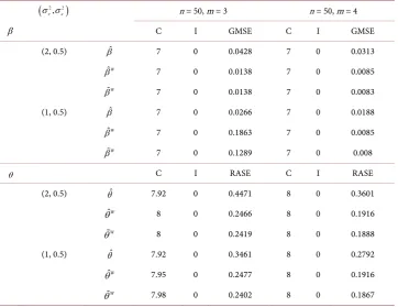
The results about variable selection, based on 100 replications, are included in Table 1.

Table 1 shows that the proposed method can select the true model quite well and leads to smaller GMSE and RASE values. Table 2 reports a satisfactory estimation for the va-riance component. As the sample increase, the performance becomes better.

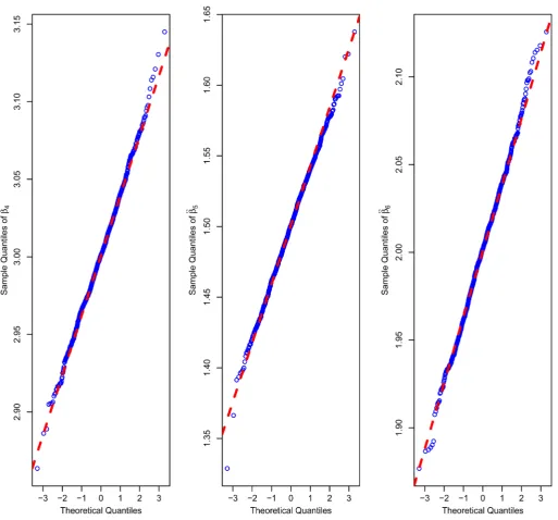
Secondly, the variance, bias and mean square error of the estimators for the nonzero parameters, denoted to be “V”, “Bias” and “MSE”, are listed in Table 3. From Table 3, all the three methods can obtain consistent estimators with small bias. Moreover, the values of “V” and “MSE” also argue that the newly proposed method and the “ideal” method can derive a more efficient estimator than the “naive” method does. What’s more, the asymptotic normality of the estimators for the parametric component is shown with Quantile-Quantile plot in Figure 1.

(7)

[image:7.595.193.556.89.368.2]

Table 1. Simulation results for the variable selection.

(

2 2

)

,

ν ε

σ σ n = 50, m = 3 n = 50, m = 4

β C I GMSE C I GMSE

(2, 0.5) _βˆ ₇ ₀ _0.0428 ₇ ₀ _0.0313

ˆW

β 7 0 0.0138 7 0 0.0085

W

β 7 0 0.0138 7 0 0.0083

(1, 0.5) _βˆ ₇ ₀ _0.0266 ₇ ₀ _0.0188

ˆW

β 7 0 0.1863 7 0 0.0085

W

β 7 0 0.1289 7 0 0.008

θ C I RASE C I RASE

(2, 0.5) _θˆ _7.92 ₀ _0.4471 ₈ ₀ _0.3601

ˆW

θ 8 0 0.2466 8 0 0.1916

W

θ 8 0 0.2419 8 0 0.1888

(1, 0.5) _θˆ _7.92 ₀ _0.3461 ₈ ₀ _0.2792

ˆW

θ 7.95 0 0.2477 8 0 0.1916

W

[image:7.595.193.558.399.529.2]

θ 7.98 0 0.2402 8 0 0.1867

Table 2. Simulation results for the estimators of the variance components 2 2

, ν ε

σ σ .

(

2 2

)

,

ν ε

σ σ n = 50, m = 3 n = 50, m = 4

2

ν

σ M V MSE M V MSE

(2, 0.5) 1.6 0.27 0.418 1.64 0.42 0.54

(1, 0.5) 0.7 0.12 0.206 0.64 0.13 0.25

2

ε

σ M V MSE M V MSE

(2, 0.5) 0.5 0.02 0.025 0.53 0.02 0.022

(1, 0.5) 0.4 0.08 0.008 0.50 0.01 0.01

Table 3. Simulation results ×100 for β β β4, 5, 6 with n = 50 and m = 3.

(

2 2

)

,

ν ε

σ σ β4 β5 β6

Var Bias MSE Var Bias MSE Var Bias MSE

(2, 0.5) _βˆ _0.498 _7.063 _0.997 _0.494 _6.456 _0.911 _0.484 _6.140 _0.861

ˆW

β _0.159 5.191 0.428 0.168 6.519 0.593 0.149 0.502 0.152

W

β

0.150 5.090 0.409 0.157 6.457 0.576 0.138 0.231 0.139 (1, 0.5) _βˆ _0.286 −4.931 0.529 0.304 −11.76 1.688 0.291 −5.826 0.630

ˆW

β _0.153 −4.128 0.323 0.152 −4.408 0.346 0.161 −5.328 0.445

W

[image:7.595.188.555.561.705.2]

(8)

[image:8.595.46.560.66.544.2]

Figure 1. Q-Q plot of the estimator ˆ4, ˆ5 ,ˆ6

W W W

β β β .

Example 2. To illustrate the effectiveness of the proposed estimation procedure, we shall apply it to the analysis of a longitudinal AIDS data set, which is reported by [18]

and comprises HIV status of 283 homosexual males who were infected with HIV dur-ing a follow-up period between 1984 and 1991. The focus in this application is to probe into the trend of the mean CD4 percentage depletion over time and evaluate the effects of cigarette smoking, preHIV infection CD4 percentage and age at infection on the mean CD4 percentage after infection.

For the jth measurement of the ith subject, let Yij be the mean CD4 percentage, tij

(9)

[image:9.595.236.513.65.340.2]

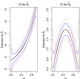
Figure 2. The estimated average curve for the nonparametric component θ1

( ) ( )

⋅ ,θ2 ⋅ and their

95% pointwise confidence interval with three coincident curves being the estimated ones for the nonparametric component, and the red dotted, the coincident solid and dotted-dashed ones be-ing the estimated confidence intervals by the “naive”, the “ideal” and the proposed method, re-spectively.

2 ,2 ,1.

i i

X =X Z_i_,1 be the centered age at HIV infection and Zi,2=Zi2,1. Let Zi,3 be the smoking status taking a value of 1 or 0. Hence, assume the following model

( )

T T

0 ,1 1 ,2 2( ) ,3 3 ,1 1 ,2 2 ,

ij ij ij ij ij ij ij ij ij ij i ij

Y =θ t +Z θ t +Z θ t +Z θ t +X β +X β ν ε+ + (20)

where the baseline of CD4 percentage θ0

( )

t is used to represent the mean CD4

per-centage of t years after the infection. The random effect νi, representing the

with-in-subject correlation, is also included in the assumed model.

By the analysis, there are two variables θ0

( )

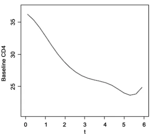
t and Xi,1 with nonzero estimators, which indicate the significant effect on the response variable Yij. Other variables’

coef-ficients are zero and have no significant effect. Moreover, the estimated curve in Figure 3

shows the trend of the mean CD4 percentage depletion over time.

5. Conclusion and Discussion

(10)

Figure 3. The estimators for the mean CD4 percentage θ0

( )

t ,

indicating the changing tendency with t.

model under a more general within-subject covariance matrix.

Acknowledgements

This work was partially supported by the National Statistical Science Research Project of China [Grant No. 2014LZ14 and 2015LZ27] and the Yancheng Teachers’ Professor and Doctors’ Research Project [Grant No. 14YSYJB0108].

References

[1] Hastie, T. and Tibshirani, R. (1993) Varying Coefficient Models. Journal of the Royal Statis-tical Society: Series B, 55, 757-796.

[2] Ahmad, I., Leelahanon, S. and Li, Q. (2005) Efficient Estimation of a Semiparametric Par-tially Linear Varying Coefficient Model. Ann. Statist., 33, 258-283.

http://dx.doi.org/10.1214/009053604000000931

[3] Pang, Z. and Xue, L.G. (2012) Estimation for the Single-Index Models with Random Effects.

Computational Statistics and Data Analysis, 56, 1837-1853.

http://dx.doi.org/10.1016/j.csda.2011.11.007

[4] Xue, L.G. and Zhu, L.X. (2007) Empirical Likelihood for a Varying Coefficient Model with Longitudinal Data. Journal of the American Statistical Association, 102, 642-652.

http://dx.doi.org/10.1198/016214507000000293

[5] Zhao, P.X. and Xue, L.G. (2010) Variable Selection for Semiparametric Varying Coefficient Partially Linear Errors-in-Variable Models. Journal of Multivariate Analysis, 101, 1872- 1883. http://dx.doi.org/10.1016/j.jmva.2010.03.005

[6] Ruckstuhl, A.F., Welsh, A.H. and Carroll, R.J. (2000) Nonparametric Function Estimation of Estimation of the Relationship between Two Repeatedly Measurement Variables. Statis-tica Sinica, 10, 51-71.

[image:10.595.252.495.64.280.2]

(11)

[8] Su, L. and Ullah, A. (2007) More Efficient Estimation of Nonparametric Panel Data Models with Random Effects. Economics Letters, 96, 375-380.

http://dx.doi.org/10.1016/j.econlet.2007.02.018

[9] You, J. and Zhou, X. (2009) Partially Linear Models and Polynomial Spline Approximations for the Analysis of Unbalanced Panel Data. Journal of Statistical Planning and Inference, 139, 679-695. http://dx.doi.org/10.1016/j.jspi.2007.04.037

[10] Fan, J. and Li, R. (2001) Variable Selection via Nonconcave Penalized Likelihood and Its Oracle Properties. Journal of the American Statistical Association, 96, 710-723.

http://dx.doi.org/10.1198/016214501753382273

[11] Zou, H. (2006) The Adaptive Lasso and Its Oracle Properties. Journal of the American Sta-tistical Association, 101, 1418-1429. http://dx.doi.org/10.1198/016214506000000735

[12] Yuan, M. and Lin, Y. (2006) Model Selection and Estimation in Regression with Grouped Variables. Journal of the Royal Statistical Society: Series B, 68, 49-67.

http://dx.doi.org/10.1111/j.1467-9868.2005.00532.x

[13] Zou, H. and Li, R.Z. (2008) One Steps Sparse Estimates in Noncave Penalized Likelihood Models. Annals of Statistics, 36, 1509-1533. http://dx.doi.org/10.1214/009053607000000802

[14] Liang, H. and Li, R.Z. (2009) Variable Selection for Partially Linear Models with Measure-ment Errors. Journal of the American Statistical Association, 104, 234-248.

http://dx.doi.org/10.1198/jasa.2009.0127

[15] Zhao, P.X. and Xue, L.G. (2009) Variable Selection for Semiparametric Varying Coefficient Partially Linear Models. Statistics and Probability Letters, 79, 2148-2157.

http://dx.doi.org/10.1016/j.spl.2009.07.004

[16] Li, G., Lai, P. and Lian, H. (2014) Variable Selection and Estimation for Partially Linear Single-Index Models with Longitudinal Data. Statistics & Computing, 25, 579-593.

http://dx.doi.org/10.1007/s11222-013-9447-8

[17] Johnson, B., Lin, D. and Zeng, D. (2008) Penalized Estimating Functions and Variable Se-lection in Semiparametric Regression Models. Journal of the American Statistical Associa-tion, 103, 672-680. http://dx.doi.org/10.1198/016214508000000184

[18] Kaslow, R.A., Ostrow, D.G., Detels, R., Phair, J.P., Polk, B.F. and Rinaldo, C.R. (1987) The Multicenter AIDS Cohort Study: Rationale, Organization and Selected Characteristics of the Participants. American Journal of Epidemiology, 126, 310-318.

http://dx.doi.org/10.1093/aje/126.2.310

Appendix

(12)

Submit or recommend next manuscript to SCIRP and we will provide best service for you:

Accepting pre-submission inquiries through Email, Facebook, LinkedIn, Twitter, etc. A wide selection of journals (inclusive of 9 subjects, more than 200 journals)

Providing 24-hour high-quality service User-friendly online submission system Fair and swift peer-review system

Efficient typesetting and proofreading procedure

Display of the result of downloads and visits, as well as the number of cited articles Maximum dissemination of your research work

Submit your manuscript at: http://papersubmission.scirp.org/