Munich Personal RePEc Archive
Time Preference and the Distributions of
Wealth and Income
Suen, Richard M. H.
January 2012
Online at
https://mpra.ub.uni-muenchen.de/36066/
Time Preference and the Distributions of
Wealth and Income
Richard M. H. Suen
yFirst Version: February 2010
This Version: January 2012
Abstract
This paper analyzes the connection between time preference heterogeneity and economic
in-equality. To achieve this, we extend the standard neoclassical growth model by introducing three
additional features, namely (i) heterogeneity in consumers’ discount rates, (ii) direct preferences for
wealth, and (iii) human capital formation. The second feature prevents the wealth distribution from
collapsing into a degenerate distribution. The third feature generates a strong positive correlation
between earnings and capital income across consumers. A calibrated version of the model is able
to generate patterns of wealth and income inequality that are very similar to those observed in the
United States.
Keywords: Inequality, Heterogeneity, Time Preference, Human Capital
JEL classi…cation: D31, E21, O15.
I would like to thank James Davies, Jang-Ting Guo, Karen Kopecky, Jim MacGee, Pierre-Daniel Sarte, Ping Wang, seminar participants at the University of Western Ontario, conference participants at the 2010 Midwest Macro Meetings and the 2010 CEA Annual Conference for helpful comments and suggestions.
yDepartment of Economics, 341 Mans…eld Road, Unit 1063, University of Connecticut, Storrs CT 06269-1063. Email:
1
Introduction
Empirical studies show that individuals do not discount future values at the same rate.1 Since indi-viduals’ asset accumulation and schooling choices are strongly a¤ected by the way they discount the
future, this type of heterogeneity would naturally lead to cross-sectional di¤erences in wealth and
in-come. To examine the connection between time preference heterogeneity and economic inequality, this
study develops a dynamic competitive equilibrium model in which consumers only di¤er in terms of
their discount rates. It is shown that a calibrated version of the model can generate patterns of wealth
and income inequality that are very similar to those observed in the United States.
The importance of time preference heterogeneity in explaining wealth inequality is well recognized
in existing studies. There is now a vast literature in macroeconomics that uses the incomplete markets
model of Huggett (1993, 1996) and Aiyagari (1994) to explain wealth and income inequality.2 The standard incomplete markets model, however, has di¢culty in explaining certain features of the wealth
distribution in the United States. In particular, it fails to generate a high concentration of wealth at the
top end of the wealth distribution.3 Krusell and Smith (1998) show that introducing time preference heterogeneity can signi…cantly improve the Aiyagari (1994) model in this regard. Similarly, Hendricks
(2007) shows that introducing this type of heterogeneity into the life-cycle model of Huggett (1996) can
improve the model’s ability to account for wealth inequality.
In both Krusell and Smith (1998) and Hendricks (2007), cross-sectional variation in income is
mainly driven by uninsurable idiosyncratic earnings risk, which is exogenous and independent of the
heterogeneity in discount rates. These two sources of consumer heterogeneity are then used to account
for the wide dispersion in wealth. This approach, however, ignores the e¤ects of time preferences on
lifetime earnings. Intuitively, more patient individuals are more willing to invest in …nancial assets as
well as human capital than less patient ones. A higher level of human capital then leads to a higher
level of lifetime earnings for those who are more patient. This intuition is consistent with empirical
…ndings. Lawrance (1991) and Warner and Pleeter (2001) …nd that more-educated households and
individuals tend to have lower discount rates than less-educated ones. This connection between patience
and educational attainment suggests that human capital formation may provide an additional channel
through which time preference heterogeneity can give rise to wealth and income inequality.
The main objective of this study is to explore the quantitative implications of this additional channel.
To achieve this, we generalize the standard deterministic neoclassical growth model to allow for three
important features, namely (i) heterogeneity in time preference, (ii) human capital formation, and (iii)
consumers’ direct preferences for wealth. The assumption of direct wealth preference has long been
used in economic studies. In an early paper, Kurz (1968) introduces wealth preference into the optimal
growth model and explores the long-run properties of the model. Zou (1994) interprets this type of
preference as re‡ecting the “capitalist spirit,” or the tendency to treat wealth acquisition as an end in
itself rather than a means of satisfying material needs. Cole et al. (1992) suggest that the inclusion
of …nancial wealth in consumers’ preferences can be viewed as a reduced-form speci…cation to capture
people’s concern for their wealth-induced status within society. Subsequent studies have followed these
traditions and interpreted this type of preference as either capturing the spirit of capitalism or re‡ecting
the demand for wealth-induced status. In this paper, we refer to this feature simply as wealth preference.
There is now a rapidly growing literature that explores the implications of wealth preference on a wide
range of issues, such as asset pricing, economic growth, expectations-driven business cycles, e¤ects of
…scal policy and wealth inequality.4
The main purpose of introducing wealth preference in our model is as follows. It is now well known
that the standard neoclassical growth model has di¢culty in generating realistic wealth distribution
based on di¤erences in discount rates alone. Becker (1980) shows that when consumers have
time-additive separable preferences and di¤erent constant discount rates, all the wealth in the neoclassical
world will eventually be concentrated in the hands of the most patient consumers. In other words,
the wealth distribution is degenerate and extremely unequal in the long run. Several existing studies
have identi…ed conditions under which the long-run wealth distribution is non-degenerate.5 In this study, we show that a non-degenerate wealth distribution can be obtained by assuming that consumers
4Studies that explore the implications of wealth preference on asset pricing include Bakshi and Chen (1996), and
Boileau and Braeu (2007) among others. Studies on economic growth include Zou (1994) and Smith (1999) among others. Karnizova (2010) introduces this type of preference into a neoclassical growth model with capital adjustment costs and shows that the model can generate expectations-driven business cycles. Gong and Zou (2002) and Nakamoto (2009) examine the welfare implications of …scal policy when consumers value wealth directly. Finally, Luo and Young (2009) explore the implications of wealth preference on wealth inequality. This study will be discussed in greater detail later on. 5Boyd (1990) shows that Becker’s result is no longer valid when consumers have recursive preferences. Sarte (1997)
have direct preferences for wealth. The intuition behind this result can be explained as follows. In
the original Becker (1980) model where there is no direct wealth preference, a consumer will choose to
hold a constant positive level of …nancial wealth only when the equilibrium interest rate is identical to
his discount rate. Since there is only one interest rate in the neoclassical model, it is not possible for
consumers with di¤erent discount rates to maintain constant positive level of wealth simultaneously.
In the long-run equilibrium, interest rate is equated to the lowest discount rate in the population.
Thus, only the most patient consumers would have positive asset holdings. All other consumers with
discount rate greater than the equilibrium interest rate will deplete their wealth until it reaches zero.
Thus, the long-run wealth distribution in the Becker (1980) model is extremely unequal. Introducing
direct preferences for wealth changes this result by creating some additional bene…ts of holding …nancial
assets. These additional bene…ts fundamentally change the consumers’ saving behavior. In particular,
consumers are now willing to maintain constant positive level of wealth even if the interest rate is lower
than their discount rates. These additional bene…ts not only prevent the consumers from depleting
their wealth to zero, they also induce di¤erent types of consumers to hold di¤erent levels of wealth.
Thus, the equilibrium wealth distribution is non-degenerate.
To illustrate the theoretical and quantitative implications of wealth preference, we begin with a
baseline model in which there is no human capital. In the baseline model, we adopt the same economic
environment as in Becker (1980), which features a neoclassical production technology, a complete set
of competitive markets, and consumers with di¤erent discount rates. The only modi…cation we make
to Becker’s model is the inclusion of …nancial wealth in consumers’ preferences. A calibrated version of
the baseline model is able to replicate some key features of the wealth distribution in the United States.
In particular, it is able to generate a large group of wealth-poor consumers and a very small group
of extremely wealthy ones. The baseline model, however, cannot produce large variations in earnings
across consumers. This type of variation is important in explaining income inequality because earnings
is the most important source of income in the model economy. Consequently, a model with only
time preference heterogeneity and wealth preference cannot explain the observed patterns of wealth
and income inequality simultaneously. The same problem remains even if we allow for endogenous
labor supply. Introducing human capital formation helps improve this result in two ways. First,
consumers’ earnings are now tied to their discount rates through the investment in human capital. This
across consumers. Second, introducing human capital helps create a strong positive correlation between
earnings and capital income. This happens because more patient consumers have higher earnings and
more …nancial wealth than less patient ones. This in turn generates a substantial degree of income
inequality in our model. A calibrated version of the model with all three features is able to replicate
the observed patterns of wealth and income inequality in the United States.6
The current study di¤ers from Krusell and Smith (1998) in three important ways: First, the current
study aims to explainboth wealth and income inequality using only one source of consumer
heterogene-ity, namely di¤erences in discount rates. Second, the current study takes into account the endogenous
components of labor income, namely endogenous labor hours and human capital formation. Third,
instead of assuming that individuals’ discount rates are stochastic and idiosyncratic in nature, the
current study focuses on …xed, predetermined di¤erences in discount rates across individuals.7
This study is also close in spirit to Luo and Young (2009) in the sense that both studies analyze
wealth and income inequality in the presence of wealth preference. There are two major di¤erences
between the two studies. First, the source of consumer heterogeneity is di¤erent in the two models. In
Luo and Young (2009), consumers share the same discount rate but face idiosyncratic uncertainty in
labor productivity as in the Aiyagari (1994) model. Thus, this study does not consider the e¤ects of time
preference heterogeneity on wealth and income inequality. Second, the earnings distribution in the two
models are determined by di¤erent factors. In Luo and Young (2009), earnings are jointly determined by
labor productivity shock and consumers’ labor-leisure choices. In particular, human capital formation
is not considered in their model. Despite these di¤erences in model speci…cation, both studies …nd
that wealth preference is a force that tends to reduce wealth inequality. In our model, this tendency
is manifested in two ways. First, the equilibrium wealth distribution is no longer extremely unequal
once we introduce wealth preference into Becker’s model. Second, in the quantitative analysis, we …nd
that the degree of wealth inequality decreases as we increase the coe¢cient that controls the strength
of wealth preference. Similar results are also reported in Luo and Young (2009).
6We do not claim that other factors, such as life-cycle factors, income uncertainty, precautionary savings, redistributive
taxation and transfer programs, are not important in understanding economic inequality. The main purpose of the calibration exercise is to illustrate the quantitative relevance of the mechanism captured by this model in explaining economic inequality.
7Existing studies show that predetermined factors (or ex ante heterogeneity) are at least as important as idiosyncratic
The rest of this paper is organized as follows. Section 2 describes the baseline model environment,
presents the main theoretical results, and evaluates the quantitative relevance of this model. Section
3 extends the baseline model by including endogenous labor supply. Section 4 extends the baseline
model by introducing human capital formation. Section 5 discusses the main determinants of wealth
and income inequality in the model with human capital. This is followed by some concluding remarks
in Section 6.
2
The Baseline Model
2.1 Preferences
Consider an economy inhabited by N >1 groups of in…nitely-lived agents. Each group is indexed by a subjective discount factor i;for i2 f1;2; :::; Ng: The discount factors can be ranked according to
0< 1 2 : : : N <1:Consumers within the same group are identical in all aspects. The share of type-i consumers in the population is given by i 2(0;1):The size of total population is constant
and is normalized to one, hencePNi=1 i = 1:
There is a single commodity in this economy which can be used for consumption and investment.
The consumers’ preferences are represented by
1
X
t=0
t
iu(ci;t; ki;t);
where ci;t is the consumption of a type-i consumer at time t and ki;t is the stock of physical capital
owned by the consumer at the beginning of timet:The (period) utility functionu:R2+!Ris identical
for all consumers and have the following properties:
Assumption A1 The function u(c; k) is twice continuously di¤erentiable, strictly increasing and strictly concave in (c; k): It also satis…es the Inada condition for consumption, i.e., lim
c!0uc(c; k) = 1;
whereuc(c; k) is the partial derivative with respect toc:
Assumption A2 The function u(c; k) is homogeneous of degree1 ;with >0:
Assumption A2 is imposed to ensure the existence of balanced growth equilibria. Under this
then de…ne a function :R+!Raccording to
(z) uk(z;1)
uc(z;1)
: (1)
By Assumption A1, the function ( )is continuously di¤erentiable and non-negative. We now impose some additional assumptions on this function.
Assumption A3 The function (z)de…ned by (1) is strictly increasing, with (0) = 0;and satis…es
lim
z!1 (z) =1:
Assumption A3 serves two important roles in the theoretical analysis. First, it plays a role in
ensuring the uniqueness of balanced-growth equilibrium. Second, it ensures that more patient
con-sumers would have more asset holdings than less patient ones in this type of equilibrium. The details
of these will become clear in Section 2.5. It is straightforward to check that ( ) is strictly increasing ifuck(c; k) 0:The converse, however, is not necessarily true. In other words, Assumption A3 does
not preclude the possibility of having a negative cross-derivative for some values ofc and k.8
All three assumptions stated above are satis…ed by the following functional forms which are
com-monly used in existing studies,
u(c; k) = 1 1 c
1 + k1 ; (2)
with >0and >0;and
u(c; k) = 1 1 e
h
c + (1 )k i
1 e
; (3)
withe>0; 2(0;1)and <1:9
2.2 The Consumers’ Problem
In each period, each consumer is endowed with one unit of time which is supplied inelastically to the
market. The consumers receive labor income from work and capital income from their previous savings.
8Majumdar and Mitra (1994) show that, in a model with homogeneous consumers, the sign of the cross derivative
uck(c; k)plays an important role in determining the dynamic properties of the model. In the current study, we only focus on stationary equilibria.
9The additively separable speci…cation is used in Zou (1994), Gong and Zou (2001), and Luo and Young (2009) among
All savings are held in the form of physical capital, which is the only asset in this economy. As in Becker
(1980), the consumers are not allowed to borrow in every period.
Letwtandrtbe the market wage rate and rental rate of physical capital at timet:Given a sequence
of wage rates and rental rates, the consumers’ problem is to choose a sequence of consumption and
asset holdings so as to maximize their lifetime utility, subject to the sequential budget constraints and
borrowing constraints. For each type-iconsumer, this problem can be expressed as
max
fci;t;ki;t+1g1t=0
1
X
t=0
t
iu(ci;t;ki;t)
subject to
ci;t+ki;t+1 (1 k)ki;t =wt+rtki;t; (4)
ki;t+1 0;
and the initial conditionki;0 >0:The parameter k2(0;1)is the depreciation rate of physical capital.
The consumer’s optimal choices are completely characterized by the budget constraint in (4), and
the Euler equation for consumption,
uc(ci;t;ki;t) i[uk(ci;t+1;ki;t+1) + (1 +rt+1 k)uc(ci;t+1;ki;t+1)]; (5)
which holds with equality if the borrowing constraint is not binding, i.e.,ki;t+1 >0:Introducing direct
preferences for wealth essentially creates some additional bene…ts for holding wealth. These additional
bene…ts are captured by the term uk(ci;t+1;ki;t+1) > 0 in the Euler equation. If consumers have no
direct preference for wealth, i.e.,uk(c; k) 0;then the Euler equation in (5) is identical to the one in
Becker (1980).
2.3 Production
Output is produced according to a standard neoclassical production function:
where Yt denote aggregate output at time t, Kt is aggregate capital, Lt is aggregate labor and Xt is
the level of labor-augmenting technology. We will refer to Lbt XtLt as e¤ective unit of aggregate
labor. The technological factor is assumed to grow at a constant exogenous rate so thatXt t for all
t; where 1 is the exogenous growth factor and X0 is normalized to one. The production function
F :R2
+!R+ is assumed to have all the usual properties which are summarized below.
Assumption A4 The production function F K;Lb is twice continuously di¤erentiable, strictly
increasing and strictly concave in each argument. It exhibits constant returns to scale and satis…es the
following conditions: F 0;Lb = 0for allLb 0; F(K;0) = 0 for allK 0; lim
K!0FK K;Lb =1 and
lim
K!1FK K;Lb = 0:
Since the production function exhibits constant returns to scale, we can focus on a representative
…rm whose problem is given by
max
Kt;Lt
fF(Kt; XtLt) wtLt rtKtg;
for anyt 0:The solution of this problem is completely characterized by the …rst-order conditions:
wt=XtFLb(Kt; XtLt) =XtFLb bkt;1 ; (6)
rt=FK(Kt; XtLt) =FK bkt;1 ; (7)
wherebkt Kt=(XtLt) is the level of physical capital per e¤ective unit of aggregate labor at timet:
2.4 Competitive Equilibrium
Let ct = (c1;t; c2;t; :::; cN;t) denote a distribution of consumption across groups at time t: Similarly,
de…nektas the distribution of physical capital at timet. Given an initial distributionk0;a competitive
equilibrium for this economy consists of a sequence of distributions,fct;ktg1
t=0;a sequence of aggregate
inputs,fKt; Ltg1t=0;and a sequence of prices, fwt; rtg1t=0;so that
(i) Given the pricesfwt; rtg1t=0;the allocationfci;t; ki;tg1t=0 solves a type-iconsumer’s problem.
(ii) Given the prices fwt; rtg1t=0; the aggregate inputs fKt; Ltg1t=0 solve the representative …rm’s
(iii) All markets clear in every period so that, for eacht 0;
Kt= N
X
i=1
iki;t; and
N
X
i=1
ici;t+Kt+1 (1 k)Kt=F(Kt; Xt):
In both theoretical and quantitative analyses, we con…ne our attention to balanced-growth equilibria
which are independent of the initial conditions. Thus, the initial distribution of physical capital is
irrelevant to our analyses. A balanced-growth equilibrium is formally de…ned as a sequence S =
fct;kt; Kt; Lt; wt; rtg1
t=0 such that
(i) S is a competitive equilibrium as de…ned above.
(ii) The rental rate of physical capital is stationary over time, i.e., rt=r for allt 0:
(iii) Individual consumption and asset holdings, aggregate capital and wage rate are all growing at
the same constant rate. The common growth factor is given by 1:
2.5 Theoretical Results
We now provide a set of conditions under which the baseline model possesses a unique balanced-growth
equilibrium. We also show that the wealth distribution in the unique equilibrium is non-degenerate.
These results are summarized in Theorem 1. The main ideas of the proof are as follows. A
balanced-growth equilibrium is mainly characterized by a constant rental rate r which clears the market for
physical capital. Once this variable is determined, all other variables in a balanced-growth equilibrium
can be uniquely determined. Thus, it su¢ces to establish the existence and uniqueness ofr . To achieve
this, we …rst formulate the supply and demand for physical capital as a function ofr:
Denote by bkd(r) the amount of physical capital per e¤ective unit of aggregate labor that the representative …rm desires when the rental rate isr: The function bkd(r) is implicitly de…ned by
r=FK bkd;1 : (8)
Under Assumption A4, the functionbkd:R++!R+ is continuously di¤erentiable and strictly
decreas-ing. Moreover, bkd(r) approaches in…nity as r tends to zero from the right and approaches zero as r
determined bywt= twb(r);where
b
w(r) =FLb kbd(r);1 : (9)
Next, we consider the supply side of the physical capital market. Along any balanced-growth
equilibrium path, individual consumption and asset can be expressed as ci;t = tbci and ki;t = tbki;
where bci and bki are stationary over time. The values of bci and bki are determined by the consumer’s
budget constraint and the Euler equation for consumption. Along a balanced growth path with rental
rater, the budget constraint becomes
b
ci =wb(r) + r bk bki; (10)
wherebk 1 + k k;and the Euler equation can be expressed as
i
(1 k) r b
ci
b
ki
; (11)
which holds with equality ifbki >0:By Assumption A3, we have (z) 0 for all z 0:In the above
condition, z is the consumption-wealth ratio for a type-i consumer, which must be non-negative in
equilibrium. Thus, the Euler equation is valid only forr rbi;where bri = i (1 k) >0: This
essentially imposes an upper bound on the equilibrium rental rate, which ismin
i frbig=brN:
10 For any
r 2(0;brN); it is never optimal for any type of consumer to choose bki = 0:11 It follows that the Euler
equation for consumption will always hold with equality in a balanced-growth equilibrium. Combining
equations (10) and (11) gives
i
(1 k) r = b
w(r)
b
ki
+r bk : (12)
This implicitly de…nes a relationship betweenbki and r: Formally, this can be expressed as kbi =gi(r);
wheregi( ) is a continuously di¤erentiable function de…ned on (0;rbi):
1 0Ifr > b
rN;then the Euler equation will not be satis…ed for some type of consumers and sorcannot be an equilibrium rental rate.
1 1To see this, suppose the contrary that a type-iconsumer chooses to havebk
i= 0in a balanced-growth equilibrium with rental rater. Then the right-hand side of (7) would become in…nite as lim
z!1 (z) =1under Assumption A3. This clearly exceeds the left-hand side of the inequality for anyr2(0;brN)and hence gives rise to a contradiction. This also means that in order to havebki>0in equilibrium, one can replace the assumption of lim
Denote by bks(r) the aggregate supply of physical capital when the rental rate is r 2 (0;rbN):
Formally, this is de…ned as
b
ks(r) =
N
X
i=1
igi(r): (13)
Since eachgi(r)is continuously di¤erentiable on(0;brN);the functionbks(r)is also continuously
di¤er-entiable on this range. A balanced-growth equilibrium exists if there exists at least one valuer ;within
the range(0;brN);that solves the physical capital market equilibrium condition:
b
kd(r) =bks(r):
Once r is determined, all other variables in the balanced-growth equilibrium can be uniquely
de-termined. If there exists a unique value of r ; then the balanced-growth equilibrium is also unique.
Theorem 1 provides the conditions under which a unique value of r exists. The proof of this result
can be found in Appendix A.
Theorem 1 Suppose Assumptions A1-A4 are satis…ed. Suppose i 1 <1for all i2 f1; :::; Ng, and
b
kd bk >bks bk : (14)
Then there exists a unique balanced-growth equilibrium. In the unique equilibrium, all types of
con-sumers hold a strictly positive amount of capital. In addition, more patient concon-sumers would have more
consumption and hold more capital than less patient ones, i.e., i > j implies bci >cbj and bki >bkj:
We now explain the intuitions behind Theorem 1. Set = 1for the moment. In the original Becker (1980) model, where consumers have no direct preference for wealth, the Euler equation is given by
i
1
i
1 r k; (15)
with equality holds if bki > 0: The parameter i is the discount rate or rate of time preference for a
type-i consumer. This equation suggests that a consumer with no direct preference for wealth will
invest according to the following rules: (i) accumulate assets inde…nitely if the e¤ective rate of return
(r k) exceeds his rate of time preference, (ii) deplete the stock of assets until it reaches zero (the
constant positive amount of assets if the two are equal. Since there is only one e¤ective rate of return
from savings, it is not possible for di¤erent types of consumers to maintain a constant amount of assets
simultaneously. In addition, no one can accumulate assets inde…nitely in a stationary equilibrium. Thus,
the e¤ective rate of return must be equated to the lowest rate of time preference in the population.
In other words, only the most patient group of consumers will have positive asset holdings in any
stationary equilibrium. All other groups of consumers will deplete their wealth until it reaches zero.
Introducing direct preferences for wealth breaks this spell by creating some additional bene…ts of
holding wealth. These additional bene…ts fundamentally change the consumers’ saving behavior. In
particular, a consumer is now willing to maintain a constant positive level of assets even if the e¤ective
rate of return is lower than his rate of time preference. This is again evident from the Euler equation
for consumption, which can be expressed as
i (r k) =
uk bci;bki
uc bci;bki
:
Since uk bci;bki > 0; we have i > (r k) for all i: It is now possible to obtain a non-degenerate
wealth distribution because consumers with di¤erent rates of time preference can choose a di¤erent
value ofbki based on the above equation. For impatient consumers, they are willing to hold a constant
level of wealth only if they are compensated by large utility gains from wealth. Under the stated
assumptions, these gains are diminishing in bki: Thus, less patient consumers would choose a smaller
value ofbki than more patient ones.
To establish the results in Theorem 1, we have imposed two mild regularity conditions. The …rst
condition requires i 1 <1 for alli2 f1; :::; Ng:This condition is both necessary and su¢cient to ensure that the lifetime utility for all types of consumers is …nite along the balanced growth path.12 The second condition, stated in (14), ensures that the unique equilibrium rental rater is greater than
bk:According to (10),r >bkis both necessary and su¢cient to guarantee that individual consumption
and asset holdings are positively correlated in the balanced-growth equilibrium. It is important to point
out that condition (14) can be checked before solving for the equilibrium rental rate. More speci…cally,
1 2This condition is commonly used in models that allow for long-term growth in per-capita consumption. See, for
b
kd b
k can be determined by substituting r=bk into (8). For eachi2 f1;2; :::; Ng;de…nexi by
1
xi
= 1
i
:
Then,gi bk =wb bk xi and bks bk is given by
b
ks bk =wb bk N
X
i=1
ixi:
This shows that bothbkd b
k andbks bk can be explicitly related to the fundamentals of the economy.
To give a more concrete example, suppose the production function takes the Cobb-Douglas form,
F(K; XL) =K (XL)1 ; 2(0;1); (16)
and the utility function is given by (2). Then, condition (14) holds if and only if
bk >(1 )
1
"N X
i=1
i i
1#
:
2.6 Numerical Results
We now examine the extent of economic inequality that can be generated by the baseline model. To
achieve this, we have to specify the form of utility function and production function, and assign speci…c
values to the model parameters. Some of these values are chosen based on empirical …ndings. Others
are chosen to match some real-world targets. The details of this procedure are explained below.
2.6.1 Functional Forms and Parameters
In the numerical exercise, the production function is assumed to take the Cobb-Douglas form as in
(16) and the utility function is additively separable as in (2). Under this speci…cation, the parameter
captures the importance of wealth preference in the utility function. In particular, a higher value of
means that the same increase in wealth would generate a larger gain in utility. The original Becker
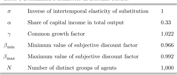
Table 1 Benchmark Parameters in Baseline Model.
Inverse of intertemporal elasticity of substitution 1
Share of capital income in total output 0.33
Common growth factor 1.022
min Minimum value of subjective discount factor 0.966
max Maximum value of subjective discount factor 0.992
N Number of distinct groups of agents 1,000
On period in the model is a year. The share of capital income in total output ( ) is 0.33. The growth rate of per-capita variables ( 1)is 2.2 percent, which is the average annual growth rate of real per-capita GDP in the United States over the period 1950-2000. In the benchmark scenario, the
parameter in the utility function is set to one. The range of subjective discount factors is chosen based
on the estimates in Lawrance (1991). Using data from the Panel Study of Income Dynamics over the
period 1974-1982, Lawrance (1991) estimates that the average rate of time preference for households
in the bottom …ve percent of the income distribution is 3.5 percent, after controlling for di¤erences in
age, educational level and race. This implies an average discount factor of 1/(1+0.035)=0.966. The
estimated rate of time preference for the richest …ve percent is 0.8 percent, which corresponds to a
discount factor of 0.992.13
In the benchmark scenario, we consider a hypothetical population of one thousand groups of
con-sumers and assume that the subjective discount factors are uniformly distributed between min = 0:966
and max= 0:992:In other words, we setN = 1;000and i= 1=N for all i:The mean discount factor
is 0.979. The choice of N is immaterial for our benchmark results. A uniform distribution is used
for the following reason. Take wealth inequality as an example. In the stationary equilibrium, wealth
inequality is driven by two types of variations: (i) variations in population shares across groups,
cap-tured byf igNi=1;and (ii) variations in the equilibrium level of asset holdings across groups, captured
by nbki
oN
i=1: By adopting a uniform distribution, we can rule out the …rst type of variation. Thus,
wealth inequality in the benchmark results is entirely driven by the cross-sectional variations in asset
holdings. The same argument applies to inequality in income. Our benchmark results then provide a
1 3To obtain these results, Lawrance (1991) estimate the Euler equation for a model without direct preferences for wealth.
clear illustration of how much inequality can be generated by the key features of the model, namely
wealth preference and heterogeneous discount factors. After presenting the benchmark results, we will
examine the e¤ects of relaxing the uniform distribution assumption and changing the values of min
and max:
In the benchmark results, we focus on the relationship between and the degree of wealth and
income inequality. To achieve this, we consider di¤erent values of ranging from 0.005 to 0.5. For each
value of ;the depreciation rate kis recalibrated so that the capital-output ratio is maintained at 3.0.
Table 1 summarizes the parameter values used in the benchmark economy.
2.6.2 Benchmark Results
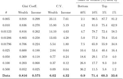
Table 2 summarizes the main …ndings of this exercise. The reported results include the Gini coe¢cients
for wealth and income, the coe¢cients of variation for wealth and income, and the shares of wealth held
by the bottom and top percentiles of the wealth distribution. The data of these inequality measures
are taken from Díaz-Giménezet al. (2011).
The results in Table 2 show a strong negative relationship between wealth inequality and the value
of : This can also be seen from Figure 1, which shows the Lorenz curves for wealth under di¤erent
values of :As approaches zero, both the Gini coe¢cient of wealth and the share of total wealth held
by the wealthiest consumers increase towards unity. This means the wealth distribution becomes more
and more concentrated when the importance of wealth preference diminishes. This result is consistent
with theoretical predictions as = 0 corresponds to the original Becker (1980) model. For small values of , the baseline model is able to generate a highly concentrated distribution of wealth with a large
group of wealth-poor consumers and a small group of extremely wealthy ones. In particular, under
certain value of ;the model is able to replicate certain key measures of wealth inequality in the United
States. For example, when = 0:01123 the Gini coe¢cient of wealth generated by the model is 0.816, when = 0:01796 the wealthiest one percent own 33.6 percent of total wealth in the model economy. These …gures coincide with the actual data reported in Díaz-Giménezet al. (2011).
As the value of increases, the wealth distribution becomes more and more equal. The intuition
behind this result is as follows. An increase in means that the same increase in asset holdings would
now generate a larger gain in utility. This has two opposing e¤ects on wealth inequality. First, a
tends to be larger for the wealth-rich than for the wealth-poor. Thus, holding other things constant,
an increase in would make the wealth distribution more unequal. Second, since aggregate savings
increase as increases, the e¤ective rate of return from savings(r k)needs to be adjusted downward
in order to maintain the same capital-output ratio. Since more patient consumers are more responsive
to interest rate changes than less patient ones, this would lower the share of total wealth owned by the
wealthiest consumers and make the wealth distribution more equal. The overall e¤ect of on wealth
inequality then depends on the relative magnitude between these two forces. Our results show that the
second e¤ect dominates under the benchmark parameter values.
Table 2 also shows that the baseline model tends to generate a relatively low degree of income
inequality. This happens because (i) earnings are identical for all consumers in this economy, and (ii)
earnings represent a sizable portion of income for most of the consumers. Table 3 reports the share of
total income from earnings for di¤erent wealth groups. When is less than 0.025, earnings accounts
for more than 80 percent of total income for the majority of the consumers.
In sum, our quantitative results show that the baseline model is able to replicate some key features
of the wealth distribution in the United States. However, it falls short of explaining income inequality.
This is partly because earnings are identical for all consumers. The two extensions considered in
Sections 3 and 4 are intended to change this feature of the baseline model.
2.6.3 Relaxing the Uniform Distribution Assumption
We now examine the e¤ects of changing the shape of the distribution of discount factors. To achieve
this, we assume that the size of each type is determined by
i = i
N
1
i 1
N
1
; with >0;
fori2 f1;2; :::; Ng:The endpoints of the distribution are …xed at their benchmark values, i.e., min = 0:966 and max = 0:992: This speci…cation of i is desirable for two reasons: (i) the skewness of the
distribution is conveniently controlled by a single parameter ; and (ii) it includes the benchmark
uniform distribution as special case (i.e., = 1): When > 1; the size of the most patient group is less than1=N and the distribution is more concentrated on low values of :The opposite is true when
more patient.
To better understand the e¤ects of on wealth inequality, we consider two experiments. In the
…rst experiment, we focus on the extent of wealth inequality under di¤erent values of :In each case,
the depreciation rate k is adjusted to maintain the capital-output ratio at 3.0. All other parameters
(including ) are …xed at their benchmark values. These results are shown in Panel (A) of Table 4.
In the second experiment, both the Gini coe¢cient for wealth and the capital-output ratio are kept
constant. This is achieved by adjusting both and k for each value of : The results of the second
experiment are summarized in Panel (B) of Table 4.
We begin by summarizing the e¤ects of changing on the distribution of discount factors. These
results are the same for both panels. Increasing from 1.0 to 2.0 raises the size of the least patient
group( 1)from 0.0010 to 0.0316, and reduces the size of the most patient group( N)by half. Because
of the skewness of the distribution, the mean value of is greater than the median value when >1. Panel (A) of Table 4 shows that the Gini coe¢cients produced by the baseline model are rather
robust to changes in the size of the most patient group. For instance, reducing N by half only raises
the Gini coe¢cients of wealth and income by 7.0 percent and 6.7 percent, respectively. The share of
total wealth owned by the wealthiest consumers are more sensitive to this change. Panel (B) shows
that once we maintain the Gini coe¢cient of wealth at the same level as in the benchmark scenario,
changing would have only a mild impact on the wealth distribution. These results show that the
main mechanism of the model is robust to changes in the shape of the distribution of discount factors.
2.6.4 Changing the Range of Discount Factors
We now examine the e¤ects of changing the range of discount factors. We maintain the uniform
distri-bution assumption as in the benchmark scenario, but consider …ve di¤erent combinations of endpoint
values. In the …rst variation, the benchmark values are reduced by 0.01 so that min = 0:956 and
max= 0:982:In the second variation, the benchmark values are reduced by 0.02. In these two
experi-ments, the range4 j max minjis the same as in the benchmark scenario. In the third and fourth
experiments, this range is reduced by half. We consider the upper half in the third experiment, i.e.,
min= 0:979and max= 0:992;and the lower half in the fourth one. In the …nal experiment, we extend
the results obtained when the capital-output ratio is kept at 3.0 and is …xed at 0.01123. Panel (B)
reports the results obtained when both the Gini coe¢cient of wealth and the capital-output ratio are
kept constant.
Two observations can be made from Panel (A). First, shifting the distribution of discount factors
while leaving the range 4 unchanged has only a small impact on the Gini coe¢cients. The share of
total wealth owned by the wealthiest consumers is also quite robust to this change. Second, wealth
inequality is positively related to the size of 4 : This is evident from the results of the last three
experiments.14 However, Panel (B) shows that once we maintain the Gini coe¢cient of wealth at
the same level, changing the range of discount factors has only a negligible impact on the wealth
distribution. These results show that the main mechanism of the baseline model is robust to di¤erent
values of minand max:They also show that the model does not rely on large values of discount factors
(i.e., very patient consumers) to generate a high concentration of wealth.
3
Endogenous Labor Supply
In this section, we extend the baseline model to include endogenous labor supply decisions. The
consumers’ period utility function is now given by
u(c; k; l) = c
1
1 +
k1
1
l1+1=
1 + 1= ; (17)
whereldenote the amount of time spent on working, >0is the intertemporal elasticity of substitution of labor, and is a positive-valued parameter. Consumers’ earnings are now endogenously determined
by their choice of working hours. The rest of the model is the same as in Section 2.
A balanced-growth equilibrium for this economy can be de…ned similarly as in Section 2.4. This
type of equilibrium now includes, among other things, a stationary distribution of labor hours which
is represented by l = (l1; l2;:::; lN): Let bkd(r) and wb(r) be the functions de…ned in (8) and (9). The
equilibrium values ofnbci;bki; li
oN
i=1 and the equilibrium rental rater are determined by
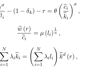
b
ci =wb(r)li+ r bk bki; (18)
i
(1 k) r = b
ci
b
ki
; (19)
b
w(r)
bci
= (li)
1
; (20)
N
X
i=1
ibki = N
X
i=1
ili
! b
kd(r); (21)
wherebk 1 + k:Equations (18) and (19) can be obtained from the consumers’ budget constraint
and their Euler equation, respectively, after imposing the balanced-growth conditions. Equation (20) is
the …rst-order condition with respect to labor. Equation (21) is the physical capital market equilibrium
condition.
We now consider the same numerical exercise as in Section 2.6. The production function again takes
the Cobb-Douglas form and the parameter values in Table 1 are used. In particular, the distribution
of discount factors is assumed to be uniform, with min = 0:966and max= 0:992:The intertemporal elasticity of substitution of labor is set to 0.4.15 As in Section 2.6, we focus on the relationship between and the degree of economic inequality. We consider the same set of values for as in Table 2. In
each case, the preference parameter is chosen so that the average amount of time spent on working
[image:21.612.239.411.59.177.2]is one-third and the depreciation rate k is chosen so that the capital-output ratio is 3.0.
Table 6 shows the inequality measures obtained under = 0:4: When comparing these to the baseline results in Table 2, it is immediate to see that they are very similar. Introducing endogenous
labor supply decisions does not change the fundamental mechanism in the baseline model. In particular,
the model continues to generate a high degree of wealth inequality when is small and a relatively
low degree of income inequality in general. A comparison to the results in Table 2 also shows that
allowing for endogenous labor supply actually lowers the Gini coe¢cient of income. This can be
explained by Figure 2, which shows the relationship between discount factor and labor supply. Most of
the consumers in this economy, except those who are very patient, choose to have the same amount of
labor. Consequently, the distribution of labor hours is close to uniform. This explains why the extended
model generates a similar degree of income inequality as the baseline model. Due to the wealth e¤ect,
wealth-rich consumers tend to work less than wealth-poor ones. This creates a negative correlation
1 5As a robustness check, we also consider two other values of this elasticity, namely 0.2 and 1.0. The results are almost
between earnings and capital income. This negative correlation in e¤ect reduces income inequality in
the model with endogenous labor supply.
4
Human Capital Formation
4.1 The Model
We now extend the baseline model to include human capital formation. Suppose in each period, each
consumer is endowed with one unit of time which can be divided between market work and on-the-job
training. Consider a type-iconsumer with human capitalhi;t at the beginning of timet:If he spends a
fractionli;t 2[0;1]of time on market work during the period, then his earnings are given bywtli;thi;t:
We refer to li;thi;t as e¤ective unit of labor hours. The variable wt is now the market wage rate for
an e¤ective unit of labor hours. The consumer also receives '(1 li;t) h&i;t units of newly produced
human capital, where' >0; 2(0;1)and& 2(0;1):His human capital at timet+ 1is then given by
hi;t+1 ='(1 li;t) h&i;t+ (1 h)hi;t; (22)
where h2(0;1)is the depreciation rate of human capital.
The consumer’s is now given by
max
fci;t;li;t;ki;t+1;hi;t+1g1t=0
1
X
t=0
t
iu(ci;t;ki;t)
subject to
ci;t+ki;t+1 (1 k)ki;t =wtli;thi;t+rtki;t;
ki;t+1 0; li;t 2[0;1];
the human capital accumulation equation in (22), and the initial conditions: ki;0 > 0 and hi;0 > 0:
The utility function is assumed to satisfy Assumptions A1-A3. The rest of the model economy remains
the same as in Section 2. In particular, long-term growth in per-capita variables is again fueled by an
exogenous improvement in labor-augmenting technology and the exogenous growth factor is 1:16
1 6Unlike the endogenous growth model considered in Lucas (1988), human capital accumulation does not serve as the
Let ht = (h1;t; :::; hN;t) denote a distribution of human capital at time t: Similarly, de…ne lt as a
distribution of labor hours at timet:Given the initial distributionsk0 andh0;a competitive equilibrium
consists of a sequence of distributions, fct;kt;lt;htg1
t=0; a sequence of aggregate inputs, fKt; Ltg
1
t=0;
and a sequence of prices,fwt; rtg1t=0;so that
(i) Given the prices, the allocationfci;t; ki;t; li;t; hi;tg1t=0 solves each type-iconsumer’s problem.
(ii) Given the prices, the aggregate inputsfKt; Ltg1t=0 solve the representative …rm’s problem in each
period.
(iii) All markets clear in every period, i.e.,
Kt= N
X
i=1
iki;t and Lt= N
X
i=1
ili;thi;t; for each t 0:
A growth equilibrium can be de…ned similarly as in Section 2.4. Speci…cally, a
balanced-growth equilibrium is a sequenceS =fct;kt;lt;ht; Kt; Lt; wt; rtg1
t=0 such that
(i) S is a competitive equilibrium as de…ned above.
(ii) The rental rate of physical capital is stationary over time, i.e., rt=r for allt 0:
(iii) The distributions of labor hours and human capital are stationary over time.
(iv) Individual consumption and asset holdings, aggregate capital and wage rate are all growing at
the same constant rate. In particular, the common growth factor is 1:
De…ne the transformed variablesbci ci;t= t andbki ki;t= t:Along any balanced growth path, the
equilibrium values ofnbci;bki; li; hi
oN
i=1 and the equilibrium rental rate r are determined by
i
(1 k) r= b
ci
b
ki
; (23)
b
ci=wb(r)lihi+ r bk bki; (24)
li
1 li
= 1 1
h
1
i
(1 h) & ; (25)
hi=
'
h
(1 li)
1 1 &
N
X
i=1
ibki= N
X
i=1
ilihi
! b
kd(r); (27)
wherebk 1 + k:Similar to the baseline model, the functionsbkd(r) andwb(r) are de…ned by (8)
and (9), respectively. Equations (23) and (24) can be obtained from the Euler equation for consumption
and the consumers’ budget constraint, after imposing the balanced-growth conditions. Equations (25)
and (26) can be obtained from the …rst-order conditions with respect toli;t andhi;t+1;and the human
capital accumulation equation. Equation (27) is the physical capital market equilibrium condition. The
mathematical derivations of (23)-(27) are shown in Appendix B.
The main theoretical results in Section 2.5 can be extended to the current model. Speci…cally, under
some mild regularity conditions, there exists a unique balanced-growth equilibrium for this economy.
This unique equilibrium has two important properties. First, the borrowing constraint is not binding
for all types of consumers. Thus, the Euler equation in (23) holds with equality for alli. Second, the
wealth distribution in the unique equilibrium is non-degenerate. The formal proof of these results are
shown in Appendix B.
Before concluding this section, we want to highlight several important features of the distributions of
labor hours and human capital. In the unique balanced-growth equilibrium, the values offli; higNi=1 can
be obtained by solving (25) and (26). These equations show that the distributions of labor hours and
human capital are non-degenerate, and are completely determined by two factors: (i) the distribution
of subjective discount factors and (ii) the parameters in the human capital accumulation process.
This has two important implications. First, the values of fli; higNi=1 are independent of the utility
function u(c; k): Thus, changing the parameters in the utility function would have no impact on the distributions of labor hours, human capital and earnings. Second, the values of fli; higNi=1 are
independent of the equilibrium rental rater and the consumers’ asset holdingsnbki
oN
i=1:Thus, in the
stationary equilibrium, the distribution of earnings is not a¤ected by the consumers’ savings decisions.
4.2 Parameter Values
In the quantitative exercise, we use the same speci…cation for production technology and utility function,
and the same distribution of discount factors as in the benchmark scenario in Section 2.6. Speci…cally,
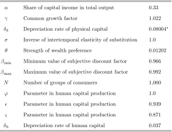
Table 7 Benchmark Parameters in Model with Human Capital.
Share of capital income in total output 0.33
Common growth factor 1.022
k Depreciation rate of physical capital 0.08004
Inverse of intertemporal elasticity of substitution 1.0
Strength of wealth preference 0.01202
min Minimum value of subjective discount factor 0.966
max Maximum value of subjective discount factor 0.992
N Number of groups of consumers 1,000
' Parameter in human capital production 1.0
Parameter in human capital production 0.939
& Parameter in human capital production 0.871
h Depreciation rate of human capital 0.037
* This …gure has been rounded o¤ to the fourth signi…cant …gure.
the results obtained under di¤erent values of : The population is divided into 1,000 groups and the
discount factors are uniformly distributed between 0.966 and 0.992.17
As for the parameter values in the human capital production function, we normalize'to unity and
set the values of and&according to the estimates reported in Heckmanet al. (1998). Using data from
the National Longitudinal Survey of Youth for the period 1979-1993, these authors …nd that the values
of and & for people who have completed at least one year of college education are 0.939 and 0.871,
respectively. For those who do not have any college education, the corresponding values are 0.945 and
0.832. We use the …rst set of parameter values in the numerical analysis because workers with college
education account for a larger share of U.S. labor force than those without college education.18 As for the depreciation rate of human capital, Heckmanet al. (1998) assume that it is zero. Other studies in
the existing literature typically …nd that this rate is greater than zero.19 In the benchmark scenario,
we set h = 0:037which is consistent with the estimate reported in Heckman (1976).
1 7The choice ofN= 1;000is again immaterial for our benchmark results. In particular, changing the number of groups to either 500 or 5,000 has virtually no impact on our benchmark results.
1 8Over the past twenty years, workers with at least some college education have accounted for an increasingly larger
share of U.S. labor force. In 1992, this type of worker represented 51.8 percent of civilian labor force (over 25 years old). This increased to 62.1 percent by the year 2010. These …gures are based on the data reported in the U.S. Statistical Abstract.
The two remaining parameters, and k;are calibrated so that the model can match two real-world
statistics. In the benchmark scenario, we choose the value of so that the Gini coe¢cient of wealth
predicted by the model is 0.816, which coincides with the value reported in Díaz-Giménezet al. (2011).
The required value of is 0.01202. Similar calibration strategy is also used in Krusell and Smith (1998),
Erosa and Koreshkova (2007), and Hendricks (2007) to determine the parameter values in the Markov
process of the random discount factor.20 The choice of , however, has no impact on the distribution
of earnings. As explained earlier, the distributions of labor hours and human capital are independent
of the utility function. Thus, the distribution of earnings in the model is not a¤ected by the preference
parameters and :The second parameter k is calibrated so that the capital-output ratio generated
by the model is 3.0. The parameter values used in the quantitative exercise are summarized in Table 7.
4.3 Benchmark Results
Table 8 summarizes the characteristics of the earnings, income and wealth distributions obtained under
the benchmark parameter values. The …rst three columns show the Gini coe¢cients, the coe¢cients of
variation and the mean-to-median ratios for the three variables. The mean-to-median ratio is intended
to measure the degree of skewness in these distributions. The rest of Table 8 shows the share of earnings,
income and wealth owned by consumers in di¤erent percentiles of the corresponding distribution.
Under the benchmark parameter values, the wealth distribution in the model economy is highly
concentrated with a large group of wealth-poor consumers and a small group of extremely wealthy
ones. For instance, the share of total wealth owned by consumers in the second quintile of the wealth
distribution is merely 1.3 percent, whereas the share owned by the wealthiest …ve percent is 58.5
percent. These …gures are very close to the actual values observed in the United States. As for the
income distribution, the model is able to generate a Gini coe¢cient and a mean-to-median ratio that
are similar to the observed values. It is also able to replicate reasonably well the share of aggregate
income owned by di¤erent quintiles of the income distribution.
As for earnings, the model predicts a more equal distribution than that observed in the data. In
the model economy, earnings-poor consumers own a larger share of total earnings than their real-world
counterparts. Consequently, the Gini coe¢cient predicted by the model is much lower than the actual
2 0Conceptually, this strategy of choosing is also no di¤erent from choosing the preference parameter in (17) to match
value.21 The big di¤erence between the model’s prediction and the actual value can be explained by two factors. First, in the actual data, a large number of households have reported negative earnings.
According to Díaz-Giménez et al. (2011), the average earnings of households in the bottom quintile
of the U.S. earnings distribution are negative due to sizable business losses. In the model economy,
earnings must be strictly positive. This restriction reduces the range and dispersion of the earnings
distribution, which in turn lowers earnings inequality in the model. Second, and more importantly,
almost all the households in the bottom quintile of the U.S. earnings distribution are not workers. As
shown in Díaz-Giménez et al. (2011) Table 4, retirees and nonworkers represent 96.9 percent of these
households, and labor income only account for 0.2 percent of their total income. If we consider only
households headed by employed worker, then the Gini coe¢cient for earnings in the United States is
0.47. This value is much closer to the one predicted by the model which assumes that all consumers
are employed.22
5
Discussion
The benchmark results in Table 8 show that our model is able to generate realistic patterns of wealth
and income inequality. To achieve this, we have extended the standard neoclassical growth model
to allow for (i) direct preferences for wealth, (ii) human capital formation, and (iii) heterogeneity in
subjective discount factors. In the above analysis, we assume that the utility function is logarithmic
(i.e., = 1) and additively separable, and the distribution of discount factors is uniform. In this section, we examine the signi…cance of each of these features in explaining wealth and income inequality. The
main objective of this exercise is to better understand the determinants of wealth and income inequality
in our model.
5.1 Strength of Wealth Preference
The purpose of this subsection is to illustrate the e¤ects of wealth preference on wealth and income
inequality in the extended model. To achieve this, we compute a series of balanced-growth equilibria
2 1Our results on earnings inequality, however, are comparable to those obtained by Pijoan-Mas (2006) and Erosa and
Koreshkova (2007). In the benchmark model of Pijoan-Mas (2006), the Gini coe¢cient and the coe¢cient of variation for the earnings distribution are 0.33 and 0.65, respectively. In the benchmark model of Erosa and Koreshkova (2007), the Gini coe¢cient of earnings is 0.289.
using di¤erent values of ranging from 0.005 to 0.5. For each value of ;the depreciation rate k is
recalibrated so that the capital-output ratio is maintained at 3.0. All other parameters values are the
same as in Table 7.
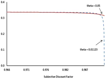
The results of this exercise are shown in Table 9.23 Similarly to the results shown in Table 2, inequality in wealth and income decrease as increases. But the decline in income inequality is much
smaller than the decline in wealth inequality. This happens because (i) consumers’ earnings are not
a¤ected by the parameter ;and (ii) for most of the consumers in this economy, earnings account for a
large fraction of their income.24 Thus, changing has only a mild impact on the income distribution.
When comparing the results in Table 2 and Table 9, we can see that removing human capital
formation from the extended model only lowers the Gini coe¢cient of wealth by 1.5 percent when
= 0:01202: In other words, wealth inequality in the extended model is mainly driven by wealth preference and the heterogeneity in discount factors.
5.2 Non-Separable Utility Function
In the existing literature, it is also common to use the following non-separable utility function,
u(c; k) =
8 > < > : 1
1 e c + (1 )k
1 e
for <1 and 6= 0;
1
1 e c k1
1 e
; for = 0;
with e > 0 and 2(0;1): Under the additively separable utility function, the Euler equation in the balanced-growth equilibrium is given by
i
(1 k) r = b
w(r)lihi
b
ki
+r bk :
Under the non-separable speci…cation, the Euler equation becomes
e
i
(1 k) r=
1 wb(r)lihi
b
ki
+r bk
1
:
2 3As explained earlier, the earnings distribution is independent of :Thus, for all the cases considered in Table 9, the earnings distribution is the same as in the benchmark scenario.
2 4When is 0.05 or less, earnings represent more than 70 percent of income for those in the bottom four quintiles (i.e.,
A direct comparison between these two equations suggests that they can be made identical by a
suit-able choice of parameter values. When this is imposed, the equilibrium wealth distribution and the
equilibrium rental rate will be identical under these two speci…cations of utility function.25 Formally, let bk = bk1; :::;bkN be the distribution of physical capital obtained under the additively separable
speci…cation and a common growth factor : Then the same distribution can be obtained under a
non-separable utility function with = 1 ; = 1=(1 + );and a common growth factore= 1e :26
This observation suggests that these two forms of utility function are likely to yield quantitatively
similar resultsin the balanced-growth equilibrium.27 The additively separable form is preferred because
it involves fewer parameters.
5.3 Relaxing the Uniform Distribution Assumption
We now perform the same sensitivity analysis as in Section 2.6.3. In particular, the share of each group
in the population is now determined by
i = i
N
1
i 1
N
1
; with >0;
fori2 f1;2; :::; Ng:The endpoints of the distribution are …xed at their benchmark values, i.e., min = 0:966and max= 0:992:The benchmark results in Table 8 then corresponds to the case when = 1:We consider two calibration exercises. In the …rst exercise, we examine the extent of economic inequality
under di¤erent values of : The results are shown in Panel (A) of Table 10. For each value of ; the
depreciation rate of physical capital is adjusted so as to maintain the capital-output ratio at 3.0. All
other parameters (including ) are …xed at their benchmark values. In the second exercise, both and
k are recalibrated in each case so that the two calibration targets (Gini coe¢cient of wealth and the
capital-output ratio) are the same as in the benchmark scenario. The results of the second experiment
are summarized in Panel (B) of Table 10.
Overall, the results of this exercise are similar to those obtained from the baseline model. Panel
(A) of Table 10 shows that the Gini coe¢cients produced by the model are rather robust to changes in
2 5Since the values offl
i; higNi=1are independent of the utility function, the distributions of labor hours, human capital
and earnings are also identical under these two speci…cations of utility function.
2 6In particular, our benchmark results can be obtained from a non-separable utility function with = 0;
e= 1and
= 1=(1 + 0:01202):
2 7We stress that the above argument is valid only in the balanced-growth equilibrium. The two speci…cations are likely
the size of the most patient group. More speci…cally, reducing N by half raises the Gini coe¢cients of
earnings, income and wealth by 13.6 percent, 10.8 percent and 8.5 percent, respectively. The share of
total wealth and total income owned by the richest consumers are more sensitive to this change. The
intuitions behind these results are as follows. First, consider the increase in earnings inequality. In the
stationary equilibrium, this type of inequality is driven by (i) cross-sectional variations in the population
share,f igN=1;and (ii) cross-sectional variations in human capital and labor hours,fhi; ligNi=1:As shown
in (25) and (26), the values offhi; ligNi=1 are independent of the e¤ective rate of return (r k) and
the population shares. This means changing has no impact on the values of fhi; ligNi=1: Thus, the
increase in earnings inequality that we observed in Panel (A) of Table 10 is completely driven by the
changes in f igN=1: In particular, an increase in lowers the share of very patient consumers in the
population. Since these consumers tend to have more human capital and higher earnings than the less
patient ones, a large portion of total earnings is now concentrated in the hands of fewer consumers.
Thus, the earnings distribution becomes more unequal as increases.
An increase in has a similar e¤ect on wealth inequality. Speci…cally, such an increase means that
a large portion of total wealth is now concentrated in the hands of fewer consumers. This makes the
wealth distribution more unequal. However, an increase in would also induce changes in the e¤ective
rate of return from savings. This creates a second e¤ect on wealth inequality. More speci…cally, an
increase in the share of less patient consumers leads to a decline in aggregate savings. In order to
maintain the same capital-output ratio, we need to adjust the e¤ective rate of return upward as
increases. Since more patient consumers are more responsive to interest rate changes than less patient
ones, this widens the di¤erences in asset holdings across groups and further increases wealth inequality.
As for income, since it is just the sum of earnings and capital income, income inequality increases as
earnings and wealth inequality increase.
Next, we turn to the results in Panel (B) of Table 10. Since adjusting has no e¤ect on the earnings
distribution, the Gini coe¢cients of earnings are the same as in Panel (A). When the Gini coe¢cient of
wealth is held constant, increasing from 1.0 to 2.0 raises the Gini coe¢cient of income by 6.5 percent,
which is smaller than the increase in Panel (A). The most signi…cant di¤erence between the two panels
is that, when the Gini coe¢cient of wealth is held constant, an increase in would lower the share of
total wealth and total income held by the richest consumers. This happens because we need to adjust