New Solution of Substrate Concentration in the Biosensor Response by Discrete Homotopy Analysis Method

(1)

http://dx.doi.org/10.4236/wjet.2013.13005

New Solution of Substrate Concentration in the Biosensor

Response by Discrete Homotopy Analysis Method

Seyyed Ali Madani Tonekaboni1, Ali Shahbazi Mastan Abad2, Shahab Karimi2, Mitra Shabani2

1

School of Mechanic, University of Waterloo, Ontario, Canada; 2School of Mechanics, University of Tehran, Tehran, Iran. Email: [email protected], [email protected], [email protected], [email protected]

Received June 22nd, 2013; revised July 28th, 2013; accepted August 26th, 2013

Copyright © 2013 Seyyed Ali Madani Tonekaboni et al. This is an open access article distributed under the Creative Commons At-tribution License, which permits unrestricted use, disAt-tribution, and reproduction in any medium, provided the original work is prop-erly cited.

ABSTRACT

In this article, Discrete Homotopy Analysis Method (DHAM), as a new numerical method, is employed to investigate amperometric biosensor at mixed enzyme kinetics and diffusion limitation. Mathematical modeling of the problem is developed utilizing non-Michaelis-Menten kinetics of the enzymatic reaction. Different results are obtained for different values of the dimensionless parameters described in the paper. The presented solution is then compared with the available actual and simulated results.

Keywords: Discrete Homotopy Analysis Method; Amperometric Biosensor; Mathematical Modeling; Non-Michaelis-Menten Kinetics

1. Introduction

Biosensor is a device which measures biologically rele- vant information such as oxygen electrodes, neutral in- terfaces, etc. [1]. It is also utilized as a component of the transduction mechanisms [1]. Furthermore, it has been applied as a transducer, mapping the change in bio- molecules into electrical signals [2]. Biosensors produce a signal indicative of the concentration of the measured analyte. As such, they are used in many industrial, envi- ronmental, food safety [3], and medical applications. Examples of such use are detection of pathogens [4], toxic metabolites such as mycotoxins [5], and pesticides and water contaminants such as heavy metal ions [6]. These applications showcase the wide usage and studies of biosensors and highlight the requirement of low detec-tion limits and quicker analysis with high specificity for biosensors [2]. Mathematical modeling is widely used as an important tool to investigate and optimize the analyti-cal characteristics of biosensors [9]. Investigative mono- layer membrane contained in the model biosensors are used to study the biochemical treatment of biosensors [7,8]. The mathematical model developed is based on reaction-diffusion equations including none-linear terms that relate to non-Michaelis-Mentenkinetics of the enzymatic reaction [9,10].

In addition to several numerical methods employed for

solving linear and nonlinear differential equations, there exists some analytical methods such as perturbation method [11], δ-expansion method [12], Adomian decomposition method (ADM) [13,14], and Homotopy perturbation method (HPM) [15,16]. All of the above mentioned methods including the numerical methods have certain restrictions, such as necessity for existence of small parameters, incapability of determining convergence regions, etc. One of the analytical methods proposed in the last couple of decades is homotopy analysis method (HAM) in which many of these restrictions have been omitted. In 1992, Liao introduced homotopy analysis method (HAM) for solving strongly nonlinear differential equations [17]. Using the linear property of homotopy, one can transform a nonlinear problem into an infi- nite number of linear sub-problems regardless of the existence of small parameterss in the original non-linear problem. HAM is a powerful mathematical technique and has already been applied to several nonlinear problems [16-22].

(2)

in fluid characteristics and the geometry of the problem. In addition, it needs little computational cost as a numerical method in comparison to HAM as an analytical approach. DHAM has similar advantages to continuous HAM. For instance, by means of introducing an auxiliary parameter one can adjust and control the convergence region of the solution series. This method should be employed for solving various differential equations to highlight its high capabilities in comparison with other numerical methods.

The main focus of this paper is on amperometric biosensor at mixed enzyme kinetics and diffusion limitation by utilizing DHAM as a powerfull method. Non-Micha- elis-Menten kinetics of the enzymatic reaction is used to obtain the constitutive equation of the problem. Several non-dimensional parameters are defined to the dimen-sionless equation. The obtained non-dimensional equa-tion is used to procure the mth-order deformation equa-tion as an important step towards obtaining the soluequa-tion. The h-curves obtained for several cases are illustrated in this paper to clarify the convergence region of the solu-tion. Finally, the obtained solution is analyzed to inves-tigate the effects of varying each dimensionless parame-ter in the procured equation of the problem. In addition, some of the results are compared with the actual and simulated results available in the literature [25].

2. Mathematical Modeling

Spatial dependency of enzyme kinetics on biochemical systems has recently attracted much attention by consid- ering the effect of diffusion in these processes [9,10]. The simplest scheme of non-Michaelis-Menten kinetics may for instance be described by adding to the Micha- elis-Menten scheme (2.1) the relationship of the interac- tion of the enzyme substrate complex



with an- other substrate molecule (2.2) followed by the gen- eration of non-active complex



ES

 

S



ES2





as

E S ES E P (2.1) 2

ES S ES (2.2) The reaction is sometimes said to display Michaelis- Menten kinetics in which the relationship between the rate of an enzyme catalyzed reaction and the substrate concentration takes the form

 

max

M

V S

K S



 (2.3)

where  and Vmax are the so-called “initial reaction velocity” and maximum velocity respectively.

In addition, KM is known as Michaelis constant for .

S KM and Vmax are constants at a given temperature and a given enzyme concentration.

The reactions exhibit non-Michaelis-Menten kinetics, in which the kinetic behavior does not obey the Equation

(2.3). The velocity function  for the simple reaction process without competitive inhibition is given by Pao [26] and Baronas et al. [27], which is based on the non- Michaelis-Menten hypothesis,

   

0 2

   

max

 

2

c

M i M

k E S V S

i

K S S K K S S K

 

    (2.4)

where the constants Vmax kc

 

E 0, KM and Ki are Michaelis-Menten and inhibition constants respectively. The Equation (2.4) conforms to Equation (2.3) for large values of Ki with respect to KM . On the basis of Equation (2.4), the rate is maximized by increasing the concentration. It is then said to be inhibited by the substrate. In addition, the constant Ki (which has the di- mension of a concentration) is called the substrate inhibition constant. For obtaining the rate of change of substrate concentration S S

 

,t at time t and position

  throughout the domain, the following equation given by Pao [26] is used.

  

,

S S

D S

t   t



 _ _{   }

 (2.5)

S is the substrate diffusion coefficient and

D S is

the gradient operation. On the basis of non-Michaelis- Menten kinetics, Equation (2.5) becomes

2

2 2

1 S

M i M

S S KS

D

t  S K S K K

 _  _

    (2.6)

in which K K E Kc 0 M .

In this paper, the steady state condition is accounted for and hence, Equation (2.6) is changed to the non-dimensional form [25] using the following non-dimensional parameters

2

2 2

1 S

M i M

S KS

D

S K S K K



 _

   (2.7)

2 2

, x= , K= , = , =

S M

S kL ks

u

L D K K K

ks

 _ _  _ 



 

i M ks

This results in the following non-dimensional differential equation

2

2 2 0, 0< 1 1

u Ku

u x u u



 

    (2.8)

Equation (2.8) must be solved such that it satisfies the following boundary conditions

1 at 1

0 at 0

u x

u _x

x

 



 



(2.9)

3. Analytical and Numerical Solutions

DHAM Solution

(3)

(Equation (2.8)) is obtained as the first step of DHAM’s procedure of the solution

 



 



 



 

_{ }

2 1 1 2 1 2

i i i

i

N q q q

q q q

K q x                      (3.1)

where is the node number, is the nonlinear operator, and the function is defined as

i N

 

i q 

 

0, 0 1 lim , lim i i q i i q

q u X

q u      

where is the unknown field variable at node number i, is the embedding parameter, and 0,i is the initial guess which is employed to meet the requirements of the boundary conditions. Here, 0,i is valued at “1” satisfying all the boundary conditions stated in Equation (2.9).

i u



0,1





q u

U

Through the generalizing concept of DHAM, the so- called zero-order deformation equation can be written as



1q L



i

 

q u0,iqhH Ni  i

 

q 

where h0 is the non-zero auxiliary parameter, Hi is the auxiliary function, and is the auxiliary linear operator which is chosen here as

L

 

1

2 2

i i i

i 1

f f f

f x        (3.2) Expanding in Taylor series with respect to the embedding parameter , one obtains

 

i q  q

 

0, , 1 , 0 1 ! m

i i m

m m

i

m i m

q

q u u q

q u m q          



i

With due attention to the procedure of DHAM [27], ,

m i should be chosen so as the following equation is sa- tisfied

u

 

,0 , ,

3

1 4

2

m m i m i m

u u u

u x      0 m i i 1 (3.3) If the series converges at , then the series solution is

 

i q

 q1

 

0, ,

1 1 i i m u u     



where m i, could be obtained by the so-called high

-order deformation equation. For obtaining the mth-order deformation equation, the following vector is defined as

u



0,, 1, , , ,



n  u i ui un

u

Differentiating both sides of the zero-order equation m

times with respect to and then setting , the so- called mth-order deformation equation can be obtained as

q q0





, 1, ,

m i m m i i m i m L u  u  hH R u 

where



_{  }

1

 

, 1 1

0

0, 1

1, otherwise

1 1 ! m

m i

m i m m

q m N q R m q             _ _    u

Therefore, the following relation is obtained





1

, 1 1 1

0 1

1 1

0 0

m

m i m m j m j

j j m

m j k j k m

j k

R u u u

u u u Ku

                     



u

We are free to choose the auxiliary parameter , the auxiliary function _i

h H , the initial guess 0,i, and the auxiliary linear operator so that the validity and flexibility of the DHAM solution to control the convergence region is proven. Due to the rule of solution ex- pression [27], the auxiliary function is chosen as follows

u L

1 i H 

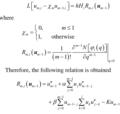
According to the DHAM, the valid region of the auxiliary parameter h for convergence of the solution series is the flat regions of h-curves. To see the proper values of h, the h-curves are plotted for different values of dimensionless parameters  , and K in Figure 1 for obtaining the valid results for the considered conditions.

4. Results and Discussion

The procedure for solving the non-dimensional equation of enzyme reaction (Equation (2.8)) which is based on the non-Michaelis-Menten kinetics theory utilizing DHAM is described in the Section 3. It is mentioned there that the mth-order deformation equation should be employed to solve the problem. As the first step towards the solution, the diagrams for variation of non-dimensional parameter u X

 

versus auxiliary parameter h for different investigated cases are illustrated in Figure 1. Then, the flat region of h-curves in each case is obtained from these diagrams.

[image:3.595.309.510.112.304.2]

(4)

(a)

(b)

(c)

[image:4.595.137.526.69.702.2]

(d)

Figure 1. Variations of u (X) versus non-dimensional pa- rameter X for (a) α = 1.0, β = 0.1, (b) α = 0.1, β = 1.0, (c) α = 10.0, β = 0.1 and (d) α = 10.0, β = 1.0.

(a)

(b)

(c)

(d)

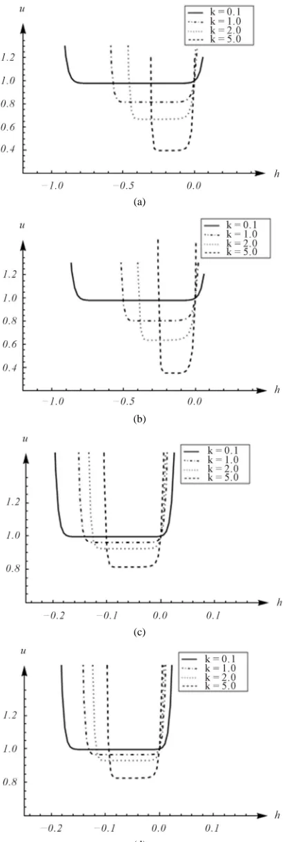
[image:4.595.71.276.84.693.2]

(5)

different locations are presented in Tables 1 and 2 for better clarifying the effects of K, as well as other non- dimensional parameter



 ,



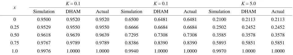
. It is clearly shown that the values of variable for lower value of  are lower than he higher ones. In addition, the spatial variation of variables which is also shown in Figure 2 is clarified. Verification of the Solution

The results of the problem obtained by employing DHAM and the results procured by simulation and actual results [25] are compared in Table 3 to show the accuracy of the presented solution. As such, the presented result in this paper can be utilized as promising data for investi-gating the behavior of the enzyme reaction in the considered conditions.

5. Conclusions

Solution to the amperometric biosensor at mixed enzyme kinetics and diffusion limitation is presented

util-izing DHAM as a new numerical method. Dimensionless equation of the problem is obtained using the mathematical modeling presented in this paper, which is based on non- Michaelis-Menten kinetics of the enzymatic reaction. Solution procedure of the non-dimensional equation of enzyme reaction is described and mth-order de- formation equation is obtained on the basis of the non-dimensional enzyme reaction equation presented in this paper. Several h-curves are dipicted to show the convergence region of the solution. Results of the solution are presented for different quantities of the dimen sionless parameters used to non-dimensionalize the enzyme reaction equation. It is shown that the most effect- tive parameter in the reaction and local dependency of the dependent variable of the problem u X

 

is K. Available results in the literature are used conclusively to prove the high accuracy of the presented solution.

[image:5.595.58.538.360.463.2]

On the basis of the presented solution for the considered problem in the area of enzyme kinetics, it can be concluded that DHAM can be employed to solve differ- Table 1. Values of non-dimensional variable u (X) at different locations for α = 1.0, β = 0.1 and α = 0.1, β = 1.0 for different values of non-dimensional parameter K.

α = 1.0, β = 0.1 α = 0.1, β = 1.0 x

K = 0.1 K = 1.0 K = 2.0 K = 5.0 K = 0.1 K = 1.0 K = 2.0 K = 5.0

[image:5.595.58.537.502.604.2]

0 0.9764 0.7831 0.6097 0.3012 0.9762 0.7675 0.5694 0.2532 0.2 0.9773 0.7916 0.6246 0.3244 0.9771 0.7767 0.5860 0.2770 0.4 0.9802 0.8172 0.6695 0.3967 0.9800 0.8044 0.6360 0.3521 0.6 0.9849 0.8601 0.7457 0.5255 0.9848 0.8507 0.7207 0.4884 0.8 0.9915 0.9209 0.8551 0.7221 0.9914 0.9159 0.8416 0.7000 1.0 1.0000 1.0000 1.0000 1.0000 1.0000 1.0000 1.0000 1.0000

Table 2. Values of non-dimensional variable u (X) at different locations for α = 10.0, β = 0.1 and α = 10.0, β = 1.0 for different values of non-dimensional parameter K.

α = 10.0, β = 0.1 α = 10.0, β = 1.0 x

K = 0.1 K = 1.0 K = 2.0 K = 5.0 K = 0.1 K = 1.0 K = 2.0 K = 5.0

0 0.9955 0.9551 0.9105 0.7790 0.9958 0.9583 0.9167 0.7924 0.2 0.9957 0.9569 0.9141 0.7878 0.9960 0.9600 0.9200 0.8007 0.4 0.9962 0.9623 0.9248 0.8142 0.9965 0.9650 0.9300 0.8255 0.6 0.9971 0.9712 0.9427 0.8583 0.9973 0.9733 0.9467 0.8670 0.8 0.9984 0.9838 0.9678 0.9202 0.9985 0.9850 0.9700 0.9252 1.0 1.0000 1.0000 1.0000 1.0000 1.0000 1.0000 1.0000 1.0000

Table 3. Comparison of results of the DHAM with simulation and actual results of the problem at different location and for different values of non-dimensional parameter K.

K = 0.1 K = 0.1 K = 5.0

x

[image:5.595.58.538.645.735.2]

(6)

ent nonlinear ordinary differential equations used to model different problems in Engineering and Science. The accuracy is clearly shown and the ablility of the aproach to control the convergence of the solution is ob- viously shown. Therefore, the employed method not only can be used to solve different complicated nonlinear problems but also can be considered as a promising numerical technique.

REFERENCES

[1] F. Scheller and F. Schubert, “Biosensors,” Vol. 7, El-sevier, Amsterdam, 1988.

[2] U. Wollenberger, F. Lisdat and F. W. Scheller, “Enzyma- tic Substrate Recycling Electrodes. Frontiers in Biosen- sorics. B and II, Practical Applications,” Birkhauser Verlag, Basel, 1997, pp. 45-70.

[3] A. Baeumner, Analytical and Bioanalytical Chemistry, Vol. 377, 2003, pp. 434-445.

[4] M. Pohanka, P. Skladal and M. Kroca, “Biosensors for Biological Warfare Agent Detection,” Defense Science

Journal, Vol. 57, No. 3, 2007, pp. 185-93.

[5] M. Pohanka, D. Jun and K. Kuca, “Mycotoxin Assay Using Biosensor Technology: A Review,” Drug and Che-

mical Toxicology, Vol. 30, No. 3, 2007, pp. 253-261. http://dx.doi.org/10.1080/01480540701375232

[6] S. Haron and A. K. Ray, “Optical Biodetection of Cad-mium and Lead Ions in Water,” Medical Engineering and Physics, Vol. 28, 2006, No. 10, pp. 978-981.

[7] A. J. Baeumner, C. Jones, C.Y. Wong and A. Price, “A Generic Sandwich-Type Biosensor with Nanomolar De-tection Limits,” Analytical and Bioanalytical Chemistry, Vol. 378, No. 6, 2004, pp. 1587-1593.

http://dx.doi.org/10.1007/s00216-003-2466-0

[8] T. Schulmeister, “Mathematical Modeling of the Dyna- mic Behavior of Ampero-Metric Enzyme Electrodes,” Se-

lective Electrode Reviews, Vol. 12, 1990, pp. 203-260. [9] R. Aris, “The Mathematical Theory of Diffusion and

Reaction in Permeable Cat-alysts. The Theory of the Steady State,” Clarendon Press, Oxford, 1975.

[10] L. K. Bieniasz and D. Britz, “Recent Developments in Digital Simulation of Electroan-Alytical Experiments,”

Polish Journal of Chemistry, Vol. 78, 2004, pp. 1195- 1219.

[11] J. D. Cole, “Perturbation Methods in Applied Mathemat-ics,” Blaisdel, Waltham, 1968.

[12] A. V. Karmishin, A. I. Zhukov and V. G. Kolosov, “Me- thods of Dynamics Calculation and Testing for Thin- Walled Structures,” Mashinostroyenie, Moscow, 1990.

[13] G. Adomian, “Solving Frontier Problems of Physics: The Decomposition Method,” Kluwer Academic Publishers, Boston, 1994.

http://dx.doi.org/10.1007/978-94-015-8289-6

[14] G. Adomian, “A Review of the Decomposition Method in Applied Mathematics,” Journal of Mathematical Analysis and Applications, Vol. 135, No. 2, 1998, pp. 501-544. http://dx.doi.org/10.1016/0022-247X(88)90170-9

[15] J. H. He, “Homotopy Perturbation Technique,” Computer

Methods in Applied Mechanics and Engineering, Vol. 178, No. 3-4, 1999, pp. 257-262.

http://dx.doi.org/10.1016/S0045-7825(99)00018-3

[16] J. H. He, “An Approximate Solution Technique depEnd-ing upon an Artificial Parameter,” Communications in Nonlinear Science and Numerical Simulation, Vol. 3, No. 2, 1998, pp. 92-97.

http://dx.doi.org/10.1016/S1007-5704(98)90070-3

[17] S. J. Liao, “The Proposed Homotopy Analysis Technique for the Solution of Nonlinear Problems,” PhD Thesis, Shanghai Jiao Tong University, 1992.

[18] S. Abbasbandy, “The Application of Homotopy Analysis Method to Nonlinear Equations Arising in Heat Trans-fer,” Physics Letters A, Vol. 360, No. 1, 2006, pp. 109- 113. http://dx.doi.org/10.1016/j.physleta.2006.07.065

[19] S. J. Liao, “Beyond Perturbation: Introduction to Homo-topy Analysis Method,” Chapman & Hall/CRC Press, Boca Raton, 2003.

http://dx.doi.org/10.1201/9780203491164

[20] J.-H. He, “Comparison of Homotopy Perturbation Me- thod and Homotopy Analysis Method,” Applied

Mathe-matics and Computation, Vol. 156, No. 2, 2004, pp. 527- 539. http://dx.doi.org/10.1016/j.amc.2003.08.008

[21] S. J. Liao, “A Short Review on the Homotopy Analysis Method in Fluid Mechanics,” Journal of Hydrodynamics,

Ser. B, Vol. 22, No. 5, 2010, pp. 882-884.

[22] S. J. Liao,” On the Homotopy Analysis Method for Non- linear Problems”, Applied Mathematics and Computation, Vol. 147, No. 2, 2004, pp. 499-513.

http://dx.doi.org/10.1016/S0096-3003(02)00790-7

[23] A. Bratsos, M. Ehrhardt and I. T. Famelis, “A Discrete Adomian Decomposition Method for Discrete Nonlinear Schrödinger Equations,” Applied Mathematics and Com-putation, Vol. 197, No. 1, 2008, pp. 190-205.

http://dx.doi.org/10.1016/j.amc.2007.07.055

[24] H. Q. Zhu, H. Z. Shu and M. Y. Ding, “Numerical Solu- tions of Partial Differential Equations by Discrete Homo- topy Analysis Method,” Applied Mathematics and Com-

putation, Vol. 216, No. 12, 2010, pp. 3592-3605. http://dx.doi.org/10.1016/j.amc.2010.05.005

[25] M. Daniel, “Dunlavy Ph.D. Candidacy Prospectus, A Ho- motopy Method for Predicting the Lowest Energy Con- formations of Proteins,” April 18, 2003.

[26] P. Manimozhia, A. Subbiahb and L. Rajendrana, “Solu-tion of Steady-State Substrate Concentra“Solu-tion in the Ac“Solu-tion of Biosensor Response at Mixed Enzyme Kinetics,”

Sen-sors and Actuators B, Vol. 147, No. 1, 2010, pp. 290-297. http://dx.doi.org/10.1016/j.snb.2010.03.008

[27] C. V. Pao, “Mathematical Analysis of Enzyme-Substrate Reaction Diffusion Insomebiochemical Systems,” Non-