Munich Personal RePEc Archive
Charitable asymmetric bidders
Olivier, Bos
LEM, University Panthéon-Assas (Paris 2)
2011
Online at
https://mpra.ub.uni-muenchen.de/31877/
Charitable Asymmetric Bidders
∗Olivier Bos†
University Panthéon-Assas (Paris 2)
This version: June, 2011
Abstract
Recent papers show that all-pay auctions are better at raising money for charity than first-price auctions with symmetric bidders and under incomplete information. Yet, this result is lost with sufficiently asymmetric bidders and under complete information. In this paper, we consider a framework on charity auctions with asymmetric bidders under some incomplete information. We find that all-pay auctions still earn more money than first-price auction. Thus, all-pay auctions should be seriously considered when one wants to organize a charity auction.
Keywords: All-pay auctions, Charity, Externalities
JEL Classification: D44, D62
∗A part of this research was done while I was visiting CORE (Université catholique de Louvain). A
Marie-Curie Fellowship from the European Commission and a grant from the European Science Foundation Activity entitled “Public Goods, Public Projects, Externalities” were gratefully acknowledged. I am indebted to Claude d’Aspremont and Cédric Wasser whose comments improved the quality of this work. I would like to thank Gabrielle Demange and Florian Morath as well as the participants of the EEA 2010, the Jamboree EDP Meeting at the LSE, the SAET Conference 2009 and seminars at Max Planck Institute (Bonn), Toulouse School of Economics, the University of Amsterdam (UvA), the University of Paris 1, the University Panthéon-Assas and the University of St Andrews for valuable comments, Thibault Fally, Martin Hellwig, Paul Heidhues, Konrad Mierendorff, Martin Ranger, Nora Szech and Stéphane Zuber for helpful conversations. All remaining errors are mine.
†University Panthéon-Assas (Paris 2), LEM, 12 place du Panthéon, 75005 Paris, France. E-mail:
1
Introduction
Fundraising activities for charitable purposes have become increasingly popular. One reason is the growing number of non-governmental organization with humanitarian or social purposes. Another one is the decrease of government participation in culture, education and related activities. The purpose of these associations are either the development and promotion of culture or aid and humanitarian services. Even in France, a country without any fundraising tradition, some organizations began to appear, such as theFrench Association of Fundraiser1
in 2007.
Commonly used mechanisms to raise money are voluntary contributions, lotteries and auctions. Even though most of the fundraisers still use voluntary contributions2
, auctions are increasingly used. Indeed, for some special events or particular situations, auctions provide a particular atmosphere. The popularity of auctions for charity purposes can also be observed by the increase in internet sites offering the sale of objects and donating a part of their
pro-ceeds to charity. Well-known examples include Yahoo! and Giving Works of eBay. Many
others have been created, such as the Pass It On Celebrity Charity Auction3 in 2003, where celebrities donated objects whose sale revenue contributed to a “charity of the month”. We can also cite cMarket Charitable Auctions Online4
created in 2002 and selected as a charity vehicle by more than 930 organizations.
Consequently, there is a growing and recent literature on charity auctions. Goeree et al.
(2005) andEngers and McManus(2007) investigate an independent private values model and show that all-pay auctions are better at raising money for charity than winner-pay auctions. Moreover, Onderstal and Schram (2009) lead a lab experiment and confirm these theoretical results. However,Carpenter et al.(2008) run a field experiment in four American preschools. In their experiments the ranking of the revenues is reversed. They attribute this result to the unfamiliarity of the participants to the mechanism and endogenous participation (see Carpen-ter et al.(2010) for a theoretical investigation of the endogenous participation). In addition, we can also investigate this question in a situation where people are different in the sense that they do not have the same believes. Indeed, Goeree et al. (2005) andEngers and McManus
(2007) assume that bidders have the same altruism parameter and valuations are drawn from the same distribution. Bos(2009) provides an answer with complete information. He investi-gates a model with complete information and heterogeneity on the bidders’ values. Then, he shows that when the asymmetry among bidders is strong enough, the ranking of revenues is reversed. In particular, winner-pay auctions outperform all-pay auctions.
1
http://www.fundraisers.fr/
2
There is further evidence of this phenomenon on the Internet with the emergence of sites such as http: //www.JustGive.org.
3
http://www.passitonline.org/
4
The point of this paper is then to determine, whether all-pay auctions are still better at raising money for charity when bidders are asymmetric under some incomplete information. If we conclude that all-pay auctions are still better with asymmetric bidders and incomplete information we should consider implementing all-pay auctions to raise money for charity in some environments. Indeed, to the best of our knowledge, all-pay auctions have never been implemented in real life for charity purposes. However, it seems easy to do it. For example, every bidder could buy a number of tickets simultaneously as in a raffle. Contrary to a raffle, though, the winner will be the buyer with the highest number of tickets in hand.
In charity auctions, bidders make their bid decisions taking into account two parameters: Their valuation for the item sold and their altruism or sensitivity to the charity purpose. In this paper we consider valuations drawn with the same distribution in an independent pri-vate values model. Then, we introduce asymmetry in the altruism parameter with complete information. As inBulow et al.(1999) and Wasser(2008), this framework has the advantage of avoiding the complexity and the narrow results of asymmetric auctions with incomplete information. In the usual asymmetric auction literature, valuations are drawn from different distributions. Changing these distributions could change the ranking of the revenue among different auction designs (for example, seeKrishna(2002)). Maskin and Riley(2000),de Fru-tos(2000) andCantillon(2008) succeed in determining the revenue ranking between first-price and second-price auctions under some conditions that the distributions should satisfy. Con-sequently, in this literature, distributions of the bidders’ value are crucial elements.
This paper is closest the spirit to Bulow et al. (1999). They investigate first-price and ascending auctions with a two bidders-common value setting. Each bidder receives an inde-pendent uniformly distributed signal that contributes to such common value and a parameter, that could be interpreted as altruism parameter to the charity purpose. These latter parame-ters are asymmetric and common knowledge. Although they apply this framework to toeholds and takeovers, it is well suited for charity. In their paper, they determine that when these pa-rameters are asymmetric and small enough, the revenue ranking could be reverse (relatively to the symmetric case) so that the first-price outperforms the ascending auction.5
Unlike them, we compare first-price to all-pay auctions in an independent private values model. The only other papers on asymmetric auctions with this kind of externalities arede Frutos (2000) and
Wasser(2008). de Frutos(2000) compares first-price and second-price auctions with altruism parameters equal to1/2and bidders’ values drawn from different distribution. Her framework is quite different to ours as she does not investigate all-pay auctions and the asymmetry con-cerns bidders values and not altruism parameters. However, dividing our all-pay auction by
5
1 minus the bidder’s altruism parameter leads to the all-pay auction in her framework with uniform distributions.6
Thus, in a technical way, our papers are connected. Wasser (2008) investigates k+ 1-price winner-pay auctions with asymmetry on the altruistic parameters. Yet, he does not compare the expected revenue among the auction design but focuses on the performance of auctions as mechanisms for partnership dissolution. Thus our papers are com-plements as they are related thanks to the existence and uniqueness of the first-price auction but differs on economic problems raised and results. In a recent paper Lu (2010) develops a methodology to deal with asymmetric externalities and presents as a leading application charity auctions. He determines an optimal mechanism such as the seller cancels the auction if he does not receive positive payments from all potential participants.
Section2sets out our simple model of two bidders with altruistic asymmetric parameters that have independent private values about the item sold. Then in Section3 and Section 4
we characterize the bidding equilibrium strategies for the all-pay auction and the first-price auction. In Section 5, we compare revenues and show that all-pay auction still outperforms first-price auction independently of level of asymmetry in their sensibility parameter. Proofs not provided straight away after the results are available in Appendix.
2
Preliminaries
Suppose two bidders take part in an auction through a fundraising event such as a charity din-ner. Each bidder is risk neutral and cares about how much she pays as well as her competitor pays in the auction. Indeed, as the amount of money will be used for a charity purpose, the bidders include in their utility function the bids paid. Thus, their bidding functions depend of two parameters: Their valuation of the object sold and their altruism or their interest for the charity purpose that the auction should finance. The more a bidder is sensitive to the charity event the higher this parameter will be. Denote as vi the valuation and asai bidder
i’s altruism parameter. Bidder valuationsv1, v2 are independently and identically distributed and we normalize them to uniform distributions on [0,1]. Moreover, the altruism parameters are common knowledge and heterogeneous such that a1 > a2. Then, bidder 1 has a higher preference for the charity purpose than bidder 2. When a bidder takes part in a charity auc-tion, she obtains a positive externality from the amount of money raised. Indeed, she hopes that the highest amount will be collected to finance the charity event. This is equivalent to a situation in which she would benefit from a percentage of the revenue collected as a return from the bids paid. In this paper we consider two auction designs: the all-pay auction, also called first-price all-pay auction, and the usual first-price auction.
In the all-pay auction the winner as well as the loser pays her own bid. Yet, each bidder
6
receives an externality from her own bid as well as from her competitor’s bid. Denote as
UA
i (vi, bi, bj;ai) the utility of bidderi
UiA(vi, bi, bj;ai) =
vi−bi+ai(bi+bj) if bi > bj
−bi
2 +ai(bi+bj) if bi < bj
vi
2 −bi+ai(bi+bj) if bi =bj
(1)
In contrast, in the first-price auction the bidder with the highest bid is the winner and pays her own bid while the loser does not pay anything. Contrary to the all-pay auction, here each bidder benefits an externality only from the winner’s bid which could be her own bid. Denote asUiF(vi, bi, bj;ai); the utility of bidder ithe follows
UiF(vi, bi, bj;ai) =
vi−bi+aibi if bi > bj aibj if bi < bj
vi
2 −bi+aibi if bi =bj
(2)
It is clear that the payment rule affects the returns that bidders obtain. In the all-pay auction, bidderi’s utility is a function of her opponent’s bid for each outcome of the auction. In the first-price auction, on the other hand, if the bidderiis the winner her payoff is independent of her opponent’s bid.
Assumption (The limit of the bidders’ altruism). Bidders are not fully altruistic.
Indeed, they strictly prefer to keep their money for personal use rather than to spend it for the charitable purpose even if they win. The limit of the bidders’ altruism is a consistent assumption.
In the all-pay auction, the limit of the bidders altruism leads to ∂UiA
∂bi (vi, bi, bj;ai)<0which
is equivalent toai <1. As bidders pay if they win as well as when they lose, the limit of the altruism requires us to compute the derivatives of the bidders’ utility in these two situations. Since the limit of the bidders’ altruism is independent of the outcome of the auction these two derivatives lead to the same result.
In the first-price auction the limit of the bidders altruism leads to ∂UiF
∂bi (vi, bi, bj;ai) < 0
which is also equivalent to ai <1. As only the winner pays in the first-price auction only the outcome where he wins matter for the altruism level.
Bidderi’s strategy is a functionα(.;ai) : [0,1]→R+in the all-pay auction and a function
inverse functions of bidder i’s strategy functions given her altruism ai.7 Notice that (αi, αj)
is a Bayesian Nash equilibrium such that its fulfill the first and the second order conditions if and only if(ϕi, ϕj)also fulfill the first and the second order conditions. The same relationship also holds in the first-price auction with(βi, βj) and(φi, φj).
3
All-Pay Auction
As we said in the preliminary section, in the all-pay auction all bidders pay their own bid. Moreover, each bidder benefits an externality from her own bid as well as her from her com-petitor. Then, using (1) we can compute the expected payoff of bidderi
EUiA(vi, bi, αj;ai) =viα−1
j (bi)−bi+ai(bi+Eαj(V)). (3)
To determine the effect of the altruism on the expected payoff we can divide (3) in two terms, the usual expected utility and the return from the charity purpose,κAi . Then,
EUiA(vi, bi, αj;ai) =viα−j1(bi)−bi+κAi (bi, αj;ai)
withκAi (bi, αj;ai) =ai(bi+Eαj(V)). Thus, if bidderidoes not take account of the termκAi ,
she would face the usual all-pay auction expected payoff.
Lemma 1. The bidders’ equilibrium strategies must be pure strategies that are continuous and strictly increasing functions.
Lemma 2. Minimum and maximum bids must be the same for both bidders so that α1(0) =
α2(0) = 0 andα1(1) =α2(1) = ¯b.
In an all-pay auction, bidders care about their bids if they win as well as when they lose. In both cases, they get a positive return from their opponent’s bid. Thus, their equilibrium bid depends on their own altruism parameter as well as on their competitor’s. An immediate con-sequence of the Lemma1is that the inverse function ofαi,ϕi, is increasing and differentiable almost everywhere on[0,¯b]. Furthermore,ϕi(0) = 0and ϕi(¯b) = 1 where¯b=α1(1) =α2(1).
To derive the equilibrium, we state here only the necessary condition while the sufficient condition is given in Appendix. Differentiating (3) with respect tobi it follows that
ϕ1(b) = 1−a1
ϕ′
2(b)
for all b∈(0,¯b] (4)
ϕ2(b) = 1−a2
ϕ′
1(b)
for all b∈(0,¯b]. (5)
Then, from (4) and (5) and using the boundary conditionsϕi(0) = 0 we get
ϕi(b)ϕj(b) = (1−ai)b+ (1−aj)bfor all b∈(0,¯b]. (6)
7
Asϕi(¯b) = 1 for all i,¯b= 1 2−a1−a2
follows from (6). Then, for some level of the altruism parameters, bidders could submit a maximum bid higher than their valuation. Indeed, this would be the case if the sum of the altruism parameters is higher than 1. Moreover, if each altruism parameter is close to 1, the maximum bid would be infinite as in the case of sym-metric bidders (seeGoeree et al.(2005)). Thus, revenue is not bounded and could potentially be infinite.
Using (5), fori= 1,2 equation (6) leads to8
ϕi(b) = 2−ai−aj 1−aj
ϕ′i(b)bfor all b∈(0,¯b].
From this we obtain an explicit solution to the inverse bid functions which characterize the unique Bayesian Nash equilibrium(ϕ1(.), ϕ2(.)):
ϕi(b) = [(2−ai−aj)b]
1−aj
2−ai−aj for all b∈(0,¯b], for i= 1,2 (7)
Proposition 1. There exists a unique Bayesian Nash equilibrium(α1, α2) such that
αi(v) = 1 2−ai−ajv
2−ai−aj
1−aj for all v
∈[0,1], i= 1,2 andi6=j.
Obviously, fora1 =a2≡awe get the symmetric Nash equilibrium
α1(v) =α2(v) = 1 2(1−a)v
2.
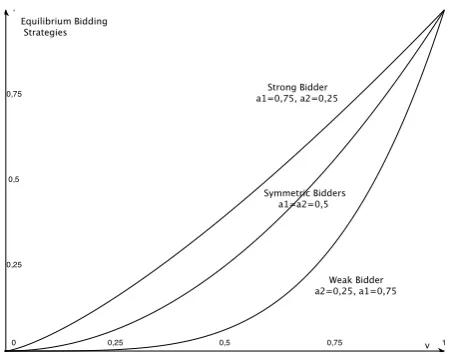
The equilibrium strategy function of bidder i is increasing in her own altruism parameter. Indeed, the more she is concerned with the charity purpose the higher her bid will be. On the other hand, the higher her opponent’s sensitivity, the less she would like to bid. A higher sensitivity leads to a higher aggressiveness which affects her bid. These results can be verified by computing the derivatives
∂αi
∂ai(v;ai, aj) =−
1
(2−ai−aj)2v 2−ai−aj
1−aj
1 +2−ai−aj 1−aj lnv
≥0
∂αi
∂aj(v;ai, aj) =
−1 + (2−ai−aj)v
2−ai−aj
1−aj 1−ai
(1−aj)2 lnv
(2−ai−aj)2 ≤0
Figure 1depicts the equilibrium bidding strategies for a1= 0,75 and a2 = 0,25.
Corollary 1. In the all-pay auction, the more altruistic bidder is the more aggressive one. More precisely, if a1 > a2 then α1(v)> α2(v) for all v∈(0,1).
8
0 0,25 0,5 0,75 1 0,25
0,5 0,75 1
Equilibrium Bidding Strategies
v Strong Bidder
a1=0,75, a2=0,25
[image:9.595.189.415.104.281.2]Weak Bidder a2=0,25, a1=0,75 Symmetric Bidders a1=a2=0,5
Figure 1: Equilibrium Bidding Strategies
4
First-Price Auction
In the first-price auction the bidder with the highest bid gets the object and pays her own bid while the loser does not pay anything (see Section 2). Moreover, each bidder experiences a positive externality from the winner’s bid. Using (2) we can then compute the expected payoff of bidderi
EUiF(vi, bi, βj;ai) = [vi−(1−ai)bi]β−1
j (bi) +ai
Z 1
β−j1(bi)
βj(v)dv (8)
(9)
Again, we can split the expected payoff in two terms. The first one is the expected payoff of the usual first-price auction and the second the return from the charity purpose, κF
i :
[vi−bi]βj−1(bi) +κFi (bi, βj;ai)
withκF
i (bi, βj;ai) =ai biβ−j1(bi) +
Z 1
βj−1(bi)
βj(v)dv
!
. As in the all-pay auction, if bidder i
does not take account the termκF
i she would face the usual first-price auction expected payoff.
Lemma 3. The bidders’ equilibrium strategies must be pure strategies that are continuous and strictly increasing functions.
Lemma 4. Minimum and maximum bids must be the same for both bidders so that β1(0) =
β2(0) = 0, β1(1) =β2(1) = ¯b and¯b∈12,1.
Lemma 5. Each bidder submit a non-negative bid inferior to her value such that βi(v) < v
As in the case of the all-pay auction, from the Lemma 3 the inverse function ofβi,φi, is increasing and differentiable almost everywhere on[0,¯b]. Furthermore,φ1(0) =φ2(0) = 0and
φ1(¯b) = φ2(¯b) = 1. Bidders could not submit a maximum bid higher than their valuation. Furthermore, the maximum bid is bounded because of the limit on the bidders’ altruism. The maximum bid in the all-pay auction is therefore higher than the one in the first-price auction.9
To derive the equilibrium, as above we state only the necessary condition while the suffi-cient condition is given in Appendix. Differentiating (8) with respect tobi it follows
φ′1(b) = 1−a2
φ2(b)−b
φ1(b) for all b∈(0,¯b] (10)
φ′2(b) = 1−a1
φ1(b)−b
φ2(b) for allb∈(0,¯b]. (11)
There is no explicit solution to this differential equation systems with our boundary condi-tions. The equations (10) and (11) and the boundary conditions define equilibrium strategies if they define the optimal decision for each bidder.
Proposition 2. The unique Bayesian Nash equilibrium(β1, β2)is characterized by the inverse
bidding functions (φ1, φ2) such that
φi(b) = (1−ai) φj(b)
φ′
j(b)
+b for all b∈[0,¯b]
which satisfies the boundary conditions φi(0) = 0, φi(¯b) = 1, for i= 1,2 andi6=j.
Fora1 =a2≡awe get the symmetric Nash equilibrium (seeEngers and McManus (2007) for details) such that βi(v) = v
2−a for i = 1,2. The maximum bids, and therefore the
expected revenue, are bounded. As in the all-pay auction we can established a strict ranking of the bidding functions.
Corollary 2. In the first-price auction, the more altruistic bidder is the more aggressive one. More precisely, if a1 > a2 then β1(v)> β2(v) for all v∈(0,1).
This result is useful to determine the shape of the bidding strategies at the equilibrium. Indeed,β1 andβ2 cannot intersect. Moreover, the equilibrium bidding strategies are concave for bidder 1 and convex for bidder 2.10
Figure 2depicts the curves of β1 andβ2.
9
This result is not obvious as for some value of the altruism parameters the maximum bid in the all-pay auction is inferior to 1. Claim1establishes this result in Section5.
10
v β1, β2
1 ¯
b
1
β2(v)
[image:11.595.179.427.113.349.2]β1(v)
Figure 2: Equilibrium Bidding Strategies
5
Revenue Comparisons
In this section we examine the performance of the all-pay and first-price auctions in terms of the expected revenue. As before we assume that bidder 1 is more concerned about the purpose of charity than bidder 2 which means thata1 > a2. Our next result describes the ranking of the equilibrium bidding strategies for each bidder.
Lemma 6. Bidders’ i bidding strategies in the all-pay and the first price auction intersect only once such that
βi(v)≥αi(v) for all v ∈[0,vi¯]and αi(v)> βi(v) for all v∈(¯vi,1], for i= 1,2 andi6=j.
To prove this result we first establish properties of the bidding strategies.
Claim 1. The maximum bid in all-pay auction is higher than is first-price auction for non-negative altruism parameters.
Proof. Let us denote by ¯bA and ¯bF the maximum bids in the all-pay and first-price auction.
Clearly, ¯bA≥1 >¯bF for all a
1+a2 ≥1. Let us assume that¯bF ≥¯bA for somea1+a2 <1. Then, by continuity there exists a value of a1 +a2 such that ¯bF = ¯bA. If this case happens with asymmetric bidders then it also happens with symmetric bidders. In the latter case,
a1+a2 =a,¯bF = 1
2−a and¯b
A= 1
2(1−a). Hence the result. k
As¯bA>¯bF and the bidding strategies are strictly increasing functions, there exists ¯vi ∈
(0,1) such that αi(¯vi) = ¯bF for i= 1,2. Then, αi(v) > βi(v) for all v ∈ [¯vi,1] for i = 1,2.
Claim 2. ϕi(b)> φi(b) andϕj(b)> φj(b) for allb close to 0.
Proof. Using L’Hôspital’s rule in (10) implies:
1−ai = lim
b→0φ
′
j(b)
φi(b)−b φj(b)
= φ′j(0) lim
b→0
φi(b)−b φj(b)
= φ′j(0) lim
b→0
φ′
i(b)−1 φ′
j(b)
= φ′i(0)−1
Thus,φ′i(0) = 2−ai for i= 1,2. As ϕ′
i(b) = (1−aj)((2−ai −aj)b) −1+ai
2−ai−aj, and ai > aj, lim
b→0ϕ′i(b) = +∞. Hence, ϕ′
i(0) > φ′i(0) for i = 1,2. Therefore, ϕi(b) > φi(b) for all b sufficiently close to 0 and βi(v)> αi(v) for all v sufficiently close to0. k
Claim 3. The inverse bidding strategies φ1 and φ2 are respectively convex and concave func-tions.
Proof. Remark that from (10) and (11) φ1 and φ2 are continuous functions and therefore differentiable. From (10) and (11) we obtain
φ′′i(b) =
1−aj
(φj(b)−b)2(φi′(b)(φj(b)−b)−(φi(b)(φ′j(b)−1))for i= 1,2and i6=j. (12)
Let us assume that φ′′
2(b) > 0 for all b ∈ [0,¯bF]. Note that φ′′1(b) < 0 is equivalent to
φ′
1(b)
φ1(b)
< φ′2(b)−1 φ2(b)−b
Using (10), this is also equivalent toφ′
2(b)>2−a2. Thus, asφ′2(0) = 2−a2
φ2 convex leads to φ1 concave. Yet, φ1 concave, φ2 convex and the boundary conditions contradict the Corollary2. Hence,φ2 cannot be convex.
Let us assume that φ2 is neither convex nor concave. Then there exists at least one inflection point b such as φ′′2(b) = 0. Denote ˜b the first inflection point. Then, φ′′2(˜b) = 0 and (12) imply φ′
1(˜b) = 2−a1. As φ′1(0) = 2−a1, φ′1 is not strictly monotone on [0,˜b] and there exists ˜˜b such as φ′′
1(˜˜b) = 0 with ˜˜b < ˜b.
11
In the same way, φ′′
1(˜˜b) = 0 and (12) imply
φ′
2(˜˜b) = 2−a2. Asφ′2(0) = 2−a2,φ′2 is not monotone on [0,˜˜b]which contradicts that˜bis the first inflection point of φ2.12 Hence,φ2 has to be either convex or concave. With a symmetric argument we get the same result forφ1.
In consequence φ′′
2(b) ≤ 0 for all b ∈ [0,b¯F]. Furthermore, φ′′1(b) ≥ 0 if and only if 2−a2 ≥φ′2(b) which is true as φ2 is concave andφ′2(0) = 2−a2. Hence, φ1 is convex. k
11
Remark that if φ′1 is constant on [0,˜b],φ
′
2 is also constant on this interval and˜bcannot be an inflection
point.
12
Remark that ifφ′
2 is constant on[0,˜˜b],φ′1 is also constant on this interval. Thus,˜˜bcannot be an inflection
Claim 4. The inverse bidding strategyϕi is a concave function.
Proof. Differentiating twice (7) leads toϕ′′
i(b) =−(1−aj)(1−ai)((2−ai−aj)b)
−3+2ai+aj
2−ai−aj for
allb∈[0,¯bA], which is negative. k
Claim 2–4 imply that the curves φi and ϕi intersect once and only once. Moreover,
ϕi(b)≥φi(b) for allb∈[0,˜bi]with˜bi <¯bF andϕi(b)< φi(b) for allb∈[˜bi,¯bF]. Furthermore,
we have shown thatαi(v)> βi(v)for allv∈[¯vi,1]withαi(¯vi) = ¯bF. This completes the proof
of Lemma6.
Let us denote eAi and eFi the expected payment of bidder i in the all-pay and first-price auctions. These expected payments areeA
i (v) =αi(v) and eFi (v) =φj(βi(v))βi(v) for all v∈
[0,1]13
. Comparing the expected payments will be useful for ranking the expected revenues.
Proposition 3. The expected payment of bidder i in the all-pay auction is greater than her expected payment in the first-price auction if her valuation is sufficiently high. Moreover, her expected payment is the same in both auctions if her valuation is sufficiently low.
The expected payment in both auctions are convex functions for bidder 2, while for bidder 1 the expected payment function is convex in the all-pay auction and concave in the first-price auction. Thus it is not clear if the expected payment of bidder ifrom the all-pay auction is greater than from the first-price auction. Indeed it could happen that for a range of middle valuations the latter outperforms the former. The next proposition determines the ranking of the expected revenue.
Proposition 4. If the bidders’ altruism parameters for charity are non-negative, the expected revenue in the all-pay auction is strictly higher than in the first-price auction.
Thus, the introduction of the asymmetry on the altruism parameters does not change the ranking of the expected revenue (Goeree et al.,2005,Engers and McManus,2007). This result was not predictable as the asymmetry can reverse the ranking of the expected revenue in first and second-price auctions (Bulow et al., 1999). Furthermore, this contradicts results with complete information (Bos, 2009). Thus, our result confirms the dominance of the all-pay auction at raising money for charity in an incomplete information framework.
Moreover, the expected revenue in the all-pay auction is given by
ERA(a1, a2) = Z 1
0
α1(v)dv+
Z 1
0
α2(v)dv
= 1
2−a1−a2
1−a2 3−a1−2a2
+ 1−a1
3−2a1−a2
13
Indeed,eF
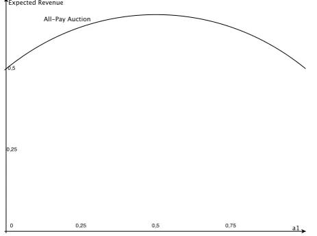
It is interesting to see how the asymmetry affects the expected revenues in the all-pay auction. In what follows, we do no longer strictly order the altruistic parameters so thata1 could be inferior as well as superior thana2. Let us denote¯a=a1+a2, such as¯a∈[0,2). Upon substitution, we can see that ERA(a1,¯a−a1)is maximized at a1 = ¯a
2 and then increasing for
a1 < ¯a2 and decreasing fora1> a¯2. For example, Figure3 depicted the situation where ¯a= 1. Then, we get the following results.
Lemma 7. The greater the asymmetry in the altruism parameters the lower the expected revenue will be in the all-pay auction.
This result is in line with results on asymmetric all-pay auctions with complete information.
Hillman and Riley (1989) determine that the expected revenue decreases when the bidders become more asymmetric.
0 0,25 0,5 0,75
0,25 0,5
!ll#Pa& !()tion ./0e)te2 Re4en(e
[image:14.595.188.420.327.499.2]a1
Figure 3: Expected Revenue of the All-Pay Auction for ¯a= 1.
Unfortunately, as we do not have explicit bidding functions in the first-price auction we cannot provide the expected revenue for this design and determine how the asymmetry affects it.
6
Conclusion
frameworkBos (2009) shows first-price auctions outperform all-pay auctions when the asym-metry among bidders is strong enough. Moreover, Carpenter et al. (2010) conclude there is no strict ranking of revenue when the participation is endogenous.
Our result confirms the one of Goeree et al. (2005) and indicates that all-pay auctions should be considered seriously to raise money for charity purposes. As we pointed out, the organization of an all-pay is unproblematic. A one-shot sale of tickets with the winner being determined by the highest number of tickets bought is equivalent to an all-pay auction.
This paper and more generally the idea that the optimal auction design for charity depends on the informational setup is good candidate for experiments in a lab. In this way one could expect to determine which elements in the knowledge of bidders are crucial to the ranking of auctions by revenue.
7
Appendix
The proofs of Lemma1 and 3are similar than the one of Lemma 1 in de Frutos(2000).
Proof of Lemma 1. First, let us show that the equilibrium bidding strategies are monotonically increasing. Denote, for a fixed ai, ¯b = αi(¯v) and b = αi(v) with v¯ ≥ v. Then, at the equilibrium, we should get
EUA
i (¯v,¯b, αj;ai)≥EUiA(¯v, b, αj;ai) and EUiA(v, b, αj;ai)≥EUiA(v,¯b, αj;ai)
which could be written
¯
vP[αj(V)<¯b] +v¯
2P[αj(V) = ¯b]−(1−ai)¯b+aiEαj(V)
≥
¯
vP[αj(V)< b] +v¯
2P[αj(V) =b]−(1−ai)b+aiEαj(V)
and
vP[αj(V)< b] + v
2P[αj(V) =b]−(1−ai)b+aiEαj(V)
≥
vP[αj(V)<¯b] + v
2P[αj(V) = ¯b]−(1−ai)¯b+aiEαj(V).
Then, subtracting the second inequality from the first one leads to(P[αj(V)<b¯]−P[αj(V)<
b])(¯v−v)≥0. Then, b≤¯b.
Let us assume there is a gap[b′, b′′]inαi(.).14
Then,αj(.)must have a gap(b′, b′′]because
for allvj bidder j would be better by bidding b′ than other bid in [b′, b′′]. Indeed, this does
not affect her probability of winning and decreases her payment. Consequently, bidderiwho
14
thought bidding b′′ would be better off submitting b′+b′′
2 ; Thus there is a contradiction and the equilibrium bidding strategies are without any gap.
Let us consider there is an atom inαi(.)such as it existsb′ withP(αi(vi) =b′)>0. Then
there is an ε >0 such that there is a gap (b′−ε, b′) inα
−i(.), leading to a contradiction to
the previous paragraph.
As the equilibrium bidding strategies are without any atom and monotonically increasing, they are strictly monotonically increasing. Furthermore the equilibrium bidding strategies are in pure strategies as there is no gap. Then, the equilibrium strategies are differentiable almost
everywhere.
Proof of Lemma 2. Assume that 0 ≤ αi(0) ≤ αj(0). Each bidder gets the same payoff by winning as well as losing. As bidders have a strict preference for a higher payoff independently of the outcome, it follows that αi(0) = αj(0) = 0. Assume that αj(1) > αi(1). Then, the bidder 1 can decrease her bid without affecting her winning probability and increasing her payoffs. Similarly,αi(1)> αj(1)cannot be part of the equilibrium. Thus, α1(1) =α2(1).
Proof of Proposition1. It is clear that at the equilibrium αi(0) = 0. Indeed, if bi = 0 the payoff of the bidder i for vi >0 is strictly inferior to the one for vi = 0. Consider now the payoff of the bidderifor allbi ∈(0,¯b].
∂UiA
∂bi (vi, bi, αj;ai) =viϕ
′
j(bi)−(1−ai)
= (vi−ϕi(bi))ϕ′j(bi).
To get the last line we used the necessary conditionϕi(bi)ϕ′j(bi) = 1−ai. Whenvi> ϕi(bi)it
follows that ∂U
A i
∂bi (vi, bi, αj;ai)>0. In a similar manner, whenvi< ϕi(bi), ∂UA
i
∂bi (vi, bi, αj;ai)<
0. Thus, ∂U
A i
∂bi (vi, αi, αj;ai) = 0. As a result, the maximum of U A
i (vi, αi, αj;ai) is achieved
forvi =ϕi(bi) and then bi =αi(vi).
Proof of Corollary1. Recall that we assume a1 > a2. As αi(x) ∈ [0,1] for all i and all x.
Then we get ϕ1(x)< ϕ2(x) for all x. The result follows.
Proof of Lemma 3. First, let us show that the equilibrium bidding strategies are monotonically increasing. Denote, for a fixedai,¯b=βi(¯v)andb=βi(v)with¯v≥v. Then, as for the all-pay auction at the equilibrium, we should get
EUiF(¯v,¯b, αj;ai)≥EUiF(¯v, b, αj;ai) and EUiF(v, b, αj;ai)≥EUiF(v,¯b, αj;ai)
which could be written
P[βj(V)<¯b][¯v−(1−ai)¯b] +P[βj(V) = ¯b][¯v2 −(1−ai)¯b] +P[βj(V)>¯b]E[βj(V)\βj(V)>¯b]
≥
P[βj(V)< b][¯v−(1−ai)¯b] +P[βj(V) =b][¯v
and
P[βj(V)< b][v−(1−ai)¯b] +P[βj(V) =b][v
2 −(1−ai)b] +P[βj(V)> b]E[βj(V)\βj(V)> b]
≥
P[βj(V)<¯b][v−(1−ai)¯b] +P[βj(V) = ¯b][v
2 −(1−ai)¯b] +P[βj(V)>¯b]E[βj(V)\βj(V)>¯b] From this we obtain (P[βj(V) < ¯b]−P[βj(V) < b])(¯v −v) ≥ 0. Then, as b ≤ ¯b. By
similar arguments to those in Lemma 1 the equilibrium bidding strategies must be gapless and atomless. In consequence the equilibrium bidding strategies are in pure strategies and strictly monotonically increasing. Then, the equilibrium strategies are differentiable almost
everywhere.
Proof of Lemma 4 and5. Assume that βi(0) < βj(0). When the valuation is 0, the payoff of losing is higher than the payoff of winning. Then, both bidders deviate and submit a bid equal to 0 such thatβ1(0) =β2(0) = 0.
Assume that¯bi >¯bj. Then bidderi wins for sure and get an expected payoff 1−bi. As ¯
bi > ¯bj, she could increase her expected payoff without changing her probability of winning by decreasing her bid to ¯bj. It follows that ¯bi = ¯bj = ¯b. Furthermore, we determine that a bidder will never submit an equilibrium bid higher than her valuationv. To see this, compare the cases where bidder i with a valuation v, either bids b=v or b=v+εwith ε >0. Using (8) it follows that
UiF(v, v, βj;ai)−UiF(v, v+ε, βj;ai) =aiv(βj−1(v)−βj−1(v+ε)) + (1−ai)εβj−1(v+ε)
+ai
Z βj−1(v+ε)
β−j1(v)
βj(x)dx
= (1−ai)εβj−1(v+ε) +ai
Z βj−1(v+ε)
β−j1(v)
βj(x)−vdx
For allx∈[β−j1(v), βj−1(v+ε)]βj(x)−v≥0. Hence,UiF(v, v, βj;ai)−UiF(v, v+ε, βj;ai)>0. Thus,βi(v)≤vfor all v∈[0,1]and¯b≤1. It follows that φi(b)≥b. In addition, as (10) and (11) leads to φi(b) = (1−ai)φφj′(b)
j(b) +b for i= 1,2 and i6= j we get φi(b) > b for all b >0.
Hence, ¯b <1.
Summing differential equations (10) and (11) it follows
φ′1(b)φ2(b) +φ
′
2(b)φ1(b)−b(φ
′
1(b) +φ
′
2(b))−(φ1(b) +φ2(b)) =−a1φ2(b)−a2φ1(b)
Intregrating this equation and using φi(¯b) = 1,
1−2¯b=−
Z ¯b
0
a1φ2(x) +a2φ1(x)dx
Hence,¯b≥ 1
Proof of Proposition2. Before solving for the equilibrium, its existence and uniqueness must be determine. Equations (10) and (11) could be written as
d
dblnφi(b)
1
1−aj = 1
1−φj(b) for i, j= 1,2, i6=j
As inde Frutos (2000), existence follows from Theorem 2 in Lebrun (1999) and uniqueness follows directly from Corollary 4 inLebrun(1999).
It is clear that at the equilibriumβi(0) = 0. Indeed, ifbi= 0 the payoff of the bidderifor
vi >0 is strictly inferior to the one for vi= 0. Consider now the payoff of the bidderifor all
bi∈(0,¯bi].
∂UF i
∂bi (vi, bi, βj;ai) = (vi−bi)φ
′
j(bi)−(1−ai)φj(bi)
= vi−bi
φi(bi)−bi(1−ai)φj(bi)−(1−ai)φj(bi)
To get the last line we used the necessary condition provided by equations (10) and (11).
φi(bi)φ′
j(bi) = 1−ai. When vi > φi(bi) it follows that ∂UF
i ∂bi
(vi, bi, βj;ai) > 0. In a similar
manner, whenvi < φi(bi), ∂U
F i
∂bi (vi, bi, βj;ai)<0. Thus, ∂UiF
∂bi (vi, βi, βj;ai) = 0. As a result,
the maximum ofUF
i (vi, βi, βj;ai)is achieved for vi =φi(bi) and then bi=βi(vi).
Proof of Corollary2. This proof is similar to the one of Proposition 4.4 inKrishna (2002). Remark that if∃y∈(0,¯b)andφ1(y) =φ2(y) =z, then (10), (11) anda1 > a2 imply that
φ′2(y) = 1−a1
z−y z < φ
′
1(y) =
1−a2
z−y z
Hence, due to properties of the inverse functions, if there exists azsuch thatβ1(z) =β2(z) =y thenβ′
2(z)> β1′(z). In consequence, β1 and β2 intersect at most once.
To prove the result let us assume the contrary. Suppose ∃x ∈ (0,1) such that β2(x) ≥
β1(x). Then either β2(v) > β1(v) for all v ∈ (0,1) or they intersect in z ∈ (0,1) and for all
x ∈ (z,1), β2(x) > β1(x). In the latter case, φ2(b) < φ1(b) for all b close to ¯b. Notice that from (10) and (11) it follows
φ1(b) =
φ2(b)
φ′
2(b)
(1−a1) +b and φ2(b) =
φ1(b)
φ′
1(b)
(1−a2) +b.
Using a1 > a2 and φ1(b) > φ2(b) we obtain φ2(b)
φ′
2(b)
> φ1(b) φ′
1(b)
for b close to ¯b. Therefore,
φ2(b)> φ1(b); hence a contradiction.15
15
Asφi(¯b) = 1, φi(0) = 0andφ′i(b)>0it follows that
φ2(b)
φ′
2(b)
> φ1(b) φ′
1(b)
impliesφ2(b)> φ1(b). That can be
shown as the dominance in terms of the reverse hazard rate implies the stochastic dominance (seeKrishna
Proof of Proposition3. The expected payment of the bidder 1 from the first-price auction is given by eF
1(v) =φ2(β1(v))β1(v). Then, eF1(0) = 0 and eF1(1) = ¯bF. As β1 and φ2 are both positive, increasing and concave functions andeF
1 is the composition and the product of them,
eF1 is also increasing and concave. Moreover, eF1′(0) = α′
1(0) and eF1(1) < α1(1). As eA1 is convex, the result follows.
Due to the same technical arguments, it follows thateA
2 andeF2 are both convex functions. In addition,eF′
2 (0) =α′2(0),eF2(0) =α2(0) = 0 andeF2(1)< α2(1). Proposition3 follows.
Proof of Proposition 4. Before showing the result, let us establish inequality (13).
Claim 5.
Z 1
0
x2 2 β
′
i(x)dx≥
Z 1 0 x2 2 dx Z 1 0
βi′(x)dxfor i= 1,2 (13)
Proof. β′
2 is an increasing function. Then, for i= 2(13) is a special case of the Chebyshev’s inequality for monotone functions. Yet, this inequality cannot be applied for i = 1 as β′
1
is decreasing. However, (13) is equivalent to
Z 1
0
x2 2 (β
′
1(x)−¯bF)dx. Then, let us show that
β′
1(x) ≥¯bF for all x ∈ [0,1]. Moreover, β1′(x) ≥ β1′(1) and ¯bF ≤ 1 2−a2
as β′
1 is decreasing and the maximum bid with asymmetric bidders cannot be higher than the maximum bid with symmetric bidders. Therefore, we need to establish thatβ′
1(1)≥
1 2−a2
. Suppose the contrary
which is equivalent toφ1(¯bF)′ ≥2−a2. This inequality is also equivalent to
1−a1
1−¯bF ≥2−a2
which leads to ¯bF ≥ 1−a2+a1
2−a2
. As 1−a2+a1 2−a2
> 1
2−a2
we obtain¯bF > 1
2−a2
; hence a
contradiction. k
Denote by∆i the difference among
Z 1
0
eAi (v)dv and
Z 1
0
eFi (v)dv such as
∆i=
Z 1
0
(αi(v)−φj(βi(v))βi(v))dv
Then,
∆2 ≥
Z 1
0
(α2(v)−φ1(β2(v))β2(v))dv (14)
= ¯bA−
Z 1
0
vα2(v)dv− ¯bF
2 + Z 1 0 v2 2β ′
2(v)dv (15)
Using Corollary 2 v ≥ φ1(β2(v) and then (14) follows. Integrating by parts we obtain (15). In addition for the bidder 1,
∆1 = ¯bA−
Z 1
0
vα1(v)dv− ¯
bF
2 +
Z 1
0
β1′(v)
Z 1
0
φ2(β1(x))dx
dv (16)
≥¯bA−
Z 1
0
vα1(v)dv− ¯
bF
2 +
Z 1
0
β1′(v)v 2
Integrating by parts we obtain equation (16) and, from Corollary 2, equation (17). Thus for
i= 1,2,
∆i ≥¯bA−
Z 1
0
vαi(v)dv−¯b F
3 (18)
≥ 2 1
−a1−a2 −
1
3−2aj −ai −
1 3(2−a2)
(19)
Using the Claim5, (15) and (17) lead to (18). To get (19) we use the fact that the maximum bid with asymmetric bidders cannot be higher than the maximum bid with symmetric bidders. Then it follows
∆1 =
5a1−a21−3a1a2−2a2+a22 3(2−a2)(2−a1−a2)(3−a1−2a2) ∆2 =
a1−2a21+ 2a2−a22
3(2−a2)(2−a1−a2)(3−2a1−a2)
and∆1+ ∆2≥ δ(a1, a2)
3(2−a2)(2−a1−a2)(3−2a1−a2)(3−a1−2a2)
withδ(a1, a2) = (3−a1−2a2)(a1−2a21+ 2a2−a22) + (3−2a1−a2)(5a1−a21−3a1a2−2a2+a22). Let us show that the functionδ(a1, a2) is positive for alla1 givena2 fixed anda1 > a2.
First, note that for each value of a2 inferior to a1, the minimum and the maximum of the function δ are given byδ(a2, a2) = 18(−1 +a2)2a2 >0 and δ(1, a2) = 2−3a2+a32 >0.
Moreover, ∂δ
∂a1
(a1, a2) = 2[6a21 +a1(11a2 −20) + 9−7a2 +a22]. Then, to determine the monoticity ofδ givena2 requires the determination of the sign of the polynomial
6a21+a1(11a2−20) + 9−7a2+a22 (20)
The discriminant of the equation (20) is 85a22 −188a2+ 76 and thus non-positive for all
a2 > a2 ≡ 94−2
√
594
85 ∼0,532. Therefore, for all a1 ∈ (a2,1) given a2 > a2 the function δ is increasing in a1. Hence, ∆1+ ∆2 >0.
Yet, whena2 ≤a2equation (20) could positive as well as negative. Indeed, (20) is positive for all a1 ≤ a1 and non-positive for all a1 > a1 with a1 ≡
20−11a2+√85a22−188a2+76
12 . Note
that a1 is positive but superior to 1 when a2 > ˜a2 ≡ −1+
√
13
6 ∼ 0,4342. Then, we have to distinguish 2 cases.
• For all a1 ∈ (0,1) given a2 < a˜2, δ is increasing for a1 ∈ (0, a1] and decreasing for
a1 ∈[a1,1). It follows that∆1+ ∆2>0.
• For all a1∈[˜a2,1)such as a2∈[˜a2, a2],δ is increasing. Hence, ∆1+ ∆2 >0.
Finally, we have determined that the functionδ is non-negative for all a1 given each value of
References
Bos, O. (2009), Charity auctions for the happy few. Cologne Working Paper Series.
Bulow, J., Huang, M. and Klemperer, P. (1999), ‘Toeholds and takeovers’,Journal of Political Economy107, 427–454.
Cantillon, E. (2008), ‘The effect of bidders’ asymmetries on expected revenue in auctions’,
Games and Economic Behavior 62, 1–25.
Carpenter, J., Homes, J. and Matthews, P. H. (2008), ‘Charity auctions : A field experiment’,
Economic Journal118, 92–113.
Carpenter, J., Homes, J. and Matthews, P. H. (2010), ‘Endogenous participation in charity auctions’,Journal of Public Economics 94, 921–935.
de Frutos, A. (2000), ‘Asymmetric price-benefits auctions’, Games and Economic Behavior
33, 48–71.
Engers, M. and McManus, B. (2007), ‘Charity auction’, International Economic Review
48(3), 953–994.
Goeree, J. K., Maasland, E., Onderstal, S. and Turner, J. L. (2005), ‘How (not) to raise money’,Journal of Political Economy113(4), 897–918.
Hillman, A. and Riley, J. (1989), ‘Politically contestable rents and transfers’, Economics and Policy1, 17–39.
Krishna, V. (2002),Auction Theory, Academic Press, Elsevier.
Lebrun, B. (1999), ‘First price auctionsin the asymmetric n bidder case’, International Eco-nomic Review40, 125–143.
Lu, J. (2010), Optimal auctions with asymmetric financial externalities. working paper.
Maskin, E. and Riley, J. (2000), ‘Asymmetric auctions’,Review of Economic Studies67, 413– 438.
Onderstal, S. and Schram, A. (2009), ‘Bidding to give : an experimental comparaison of auctions for charity’, International Economic Review50, 431–457.