A Pure Jump Transaction Level Price Model Yielding Cointegration, Leverage, and Nonsynchronous Trading Effects

Munich Personal RePEc Archive

A Pure-Jump Transaction-Level Price

Model Yielding Cointegration, Leverage,

and Nonsynchronous Trading Effects

Hurvich, Clifford and Wang, Yi

Stern School of Business, New York University, Stern School of

Business, New York University

5 January 2009

Online at

https://mpra.ub.uni-muenchen.de/12575/

A Pure-Jump Transaction-Level Price Model Yielding

Cointegration, Leverage, and Nonsynchronous Trading Effects

Clifford M. Hurvich

_{Yi Wang}

January 5, 2009

Abstract

We propose a new transaction-level bivariate log-price model, which yields fractional or standard cointegration. The model provides a link between market microstructure and lower-frequency obser-vations. The two ingredients of our model are a Long Memory Stochastic Duration process for the waiting times{τk}between trades, and a pair of stationary noise processes ({ek}and{ηk}) which

de-termine the jump sizes in the pure-jump log-price process. Our model includes feedback between the disturbances of the two log-price series at the transaction level, which induces standard or fractional cointegration for any fixed sampling interval ∆t. We prove that the cointegrating parameter can be consistently estimated by the ordinary least-squares estimator, and obtain a lower bound on the rate of convergence. We propose transaction-level method-of-moments estimators of the other parameters in our model and discuss the consistency of these estimators. We then use simulations to argue that suitably-modified versions of our model are able to capture a variety of additional properties and stylized facts, including leverage, and portfolio return autocorrelation due to nonsynchronous trading. The ability of the model to capture these effects stems in most cases from the fact that the model treats the (stochastic) intertrade durations in a fully endogenous way.

KEYWORDS_{: Tick Time; Long Memory Stochastic Duration; Information Share.}

∗_{Stern School of Business, New York University.}

I

Introduction

In this paper, we propose a transaction-level, pure-jump model for a bivariate price series, in which the

intertrade durations are stochastic, and enter into the model in a fully endogenous way. The model

is flexible, and able to capture a variety of stylized facts, including standard or fractional cointegration,

persistence in durations, volatility clustering, leverage (i.e.,a negative correlation between current returns

and future volatility), and nonsynchronous trading effects. In our model, all of these features observed at

equally-spaced intervals of time are derived from transaction-level properties. Thus, the model provides

a link between market microstructure and lower-frequency observations. This paper focuses on the

cointegration aspects of the model, presenting theoretical, simulation and empirical analysis.

Cointegration is a well-known phenomenon that has received considerable attention in Economics

and Econometrics. Under both standard and fractional cointegration, there is a contemporaneous linear

combination of two or more time series which is less persistent than the individual series. Under standard

cointegration, the memory parameter is reduced from 1 to 0, while under fractional cointegration the level

of reduction need not be an integer. Indeed, in the seminal paper of Engle and Granger (1987), both

standard and fractional cointegration were allowed for, although the literature has developed separately

for the two cases. Important contributions to the representation, estimation and testing of standard

cointegration models include Stock and Watson (1988), Johansen (1988, 1991), and Phillips (1991a).

Literature addressing the corresponding problems in fractional cointegration includes Dueker and Startz

(1998), Marinucci and Robinson (2001), Robinson and Marinucci (2001), Robinson and Yajima (2002),

Robinson and Hualde (2003), Velasco (2003), Velasco and Marmol (2004), Chen and Hurvich (2003a,

2003b, 2006).

A limitation of most existing models for cointegration is that they are based on a particular fixed

sampling interval ∆t,e.g.,one day, one month,etc.and therefore do not reflect the dynamics at all levels

of aggregation. Indeed, Engle and Granger (1987) assumed a fixed sampling interval. It is also possible to

build models for cointegration using diffusion-type continuous-time models such as ordinary or fractional

would fail to capture the pure-jump nature of observed asset-price processes.

In this paper, we propose a pure-jump model for a bivariate log-price series such that any

discretiza-tion of the process to an equally-spaced sampling grid with sampling interval ∆t produces fractional or

standard cointegration,i.e., there exists a contemporaneous linear combination of the two log-price series

which has a smaller memory parameter than the two individual series. A key ingredient in our model is

a microstructure noise contribution{ηk}to the log prices. In theweak fractional cointegration case, this

noise series is assumed to have memory parameter dη ∈ (−1₂,0), in the strong fractional cointegration

casedη ∈(−1,−1₂) while in the standard cointegration case dη =−1. In all three cases, the reduction

of the memory parameter is−dη. Due to the presence of the microstructure noise term, the discretized

log-price series are not Martingales, and the corresponding return series are not linear in either ani.i.d.

sequence, a Martingale-difference sequence, or a strong-mixing sequence. This is in sharp contrast to

existing discrete-time models for cointegration, most of which assume at least that the series has a linear

representation with respect to a strong-mixing sequence.

The discretely-sampled returns (i.e., the increments in the log-price series) in our model are not

Mar-tingale differences, due to the microstructure noise term. Instead, for small values of ∆tthey may exhibit

noticeable autocorrelations, as observed also in actual returns over short time intervals. Nevertheless,

the returns behave asymptotically like Martingale differences as the sampling interval ∆tis increased, in

the sense that the lag-k autocorrelation tends to zero as ∆t tends to∞ for any fixedk. Again, this is

consistent with the near-uncorrelatedness observed in actual returns measured over long time intervals.

The memory parameter of the log prices in our model is 1, in the sense that the variance of the

log price increases linearly in t, asymptotically as t → ∞. By contrast, the memory parameter of the

appropriate contemporaneous linear combination of the two log-price series is reduced to (1 +dη)<1,

thereby establishing the existence of cointegration in our model.

In order to derive the results described above, we will make use of the general theory of point processes,

and we will also rely heavily on the theory developed in Deo, Hurvich, Soulier and Wang (2007) for the

In Section II, we exhibit our pure-jump model for the bivariate log-price series. Since the two series

need not have all of their transactions at the same time points (due to nonsynchronous trading), it is not

possible to induce cointegration in the traditional way,i.e., by directly imposing in clock time (calendar

time) an additive common component for the two series, with a memory parameter equal to 1. Instead,

the common component is induced indirectly, and incompletely, by means of a feedback mechanism in

transaction time between current log-price disturbances of one asset and past log-price disturbances of

the other. This feedback mechanism also induces certain end-effect terms, which we explicitly display

and handle in our theoretical derivations using the theory of point processes. Subsection II A provides

economic justification of the model, as well as a transaction-level definition of the information share of

a market. The subsection also presents some preliminary data analysis results affirming the potential

usefulness of certain flexibilities in the model.

In Section III, we give conditions on the microstructure noise process for both fractional and standard

cointegration. These conditions are satisfied by a variety of standard time series models. In Section IV,

we present the properties of the log-price series implied by our model. In particular, we show that the

log price behaves asymptotically like a Martingale as t is increased, and the discretely-sampled returns

behave asymptotically like Martingale differences as the sampling interval ∆t is increased. In Section

V, we establish that our model possesses cointegration, by showing that the cointegrating error has

memory parameter (1 +dη). We present three separate theorems for the weak and strong fractional

cointegration and standard cointegration cases respectively. In Section VI, we show that the ordinary

least squares (OLS) estimator of the cointegrating parameterθ is consistent, and obtain a lower bound

on its rate of convergence. In Section VII, we propose an alternative cointegrating parameter estimator

based on the tick-level price series. In Section VIII, we propose a method-of-moments estimator for

the tick-level model parameters (except the cointegrating parameter θ). The method is based on the

observed tick-level returns. In Section IX, we propose a specification test for the transaction-level price

model. In Section X, we present simulation results on the OLS estimator ofθ, the tick-level cointegrating

parameter estimator ˜θ, the method of moments estimator and the proposed specification test. In Section

of strong fractional cointegration. The cointegrating parameter is estimated by both OLS regression and

the alternative tick-level method proposed in Section VII. The proposed specification test is implemented

on the data. Interesting results are observed that are consistent with the existing literature about price

discovery process in a market-dealer market. We then consider the information content of buy trades

versus sell trades in different market environments. In Section XII, we demonstrate, largely through

simulations, that modified versions of our model can reproduce two additional important stylized facts:

leverage, and portfolio return autocorrelation due to nonsynchronous trading. We trace these clock-time

properties to their tick-time source. In Section XIII, we provide some remarks and discuss possible

further generalizations of our model and related future work. In Section XIV we present details on the

method-of-moments estimator, establish its consistency, and propose an alternative estimator. Section

XV presents proofs.

II

A Pure-Jump Model For Log Prices

Before describing our model, we provide some background on transaction-level modeling. Currently, a

wealth of transaction-level price data is available, and for such data the (observed) price remains constant

between transactions. If there is a diffusion component underlying the price, it is not directly observable.

Pure-jump models for prices thus provide a potentially appealing alternative to diffusion-type models. The

compound Poisson process proposed in Press (1967) is a pure-jump model for the logarithmic price series,

under which innovations to the log price arei.i.d., and these innovations are introduced at random time

points, determined by a Poisson process. The model was generalized by Oomen (2006), who introduced

an additional innovation term to capture market microstructure.

An informative and directly-observable quantity in transaction-level data is the durations{τk}between

transactions. A seminal paper focusing on durations and, to some extent, on the induced price process,

is Engle and Russell (1998). They documented a key empirical fact, i.e., that durations are strongly

autocorrelated, quite unlike the i.i.d. exponential duration process implied by a Poisson transaction

related to the GARCH model of Bollerslev (1986). Deo, Hsieh and Hurvich (2006) presented empirical

evidence that durations, as well as transaction counts, squared returns and realized volatility have long

memory, and introduced the Long Memory Stochastic Duration (LMSD) model, which is closely related

to the Long Memory Stochastic Volatility model of Breidt, Crato and de Lima (1998) and Harvey (1998).

The LMSD model isτk =ehkǫk where {hk} is a Gaussian long-memory series with memory parameter

dτ ∈ (0,12), the {ǫk} are i.i.d. positive random variables with mean 1, and {hk}, {ǫk} are mutually

independent.

It was shown in Deo, Hurvich, Soulier and Wang (2007) that long memory in durations propagates

to long memory in the counting processN(t), whereN(t) counts the number of transactions in the time

interval (0, t]. In particular, if the durations are generated by an LMSD model with memory parameter

dτ ∈ (0,1₂), then N(t) is long-range count dependent with the same memory parameter, in the sense

that varN(t) ∼Ct2dτ+1 _{as t → ∞. This long-range count dependence then propagates to the realized}

volatility, as studied in Deo, Hurvich, Soulier and Wang (2007).

We now describe the tick-time return interactions that yield cointegration in our model. Suppose that

there are two assets, 1 and 2, and that each log price is affected by two types of disturbances when a

transaction happens. These disturbances are the value shocks{ei,k}and the microstructure noise{ηi,k},

for Asseti= 1,2. The subscripti, kpertains to thek’th transaction of asseti. The value shocks are iid

and represent permanent contributions to the intrinsic log value of the assets which, in the absence of

feedback effects, is a Martingale with respect to full information, both public and private (see Amihud

and Mendelson 1987, Glosten 1987). The microstructure shocks represent the remaining contributions

to the observed log prices, along similar lines as the noise process considered by Amihud and Mendelson

(1987), reflecting transitory price fluctuations due, for example, to liquidity impact of orders. We assume

that the m-th tick-time return of Asset 1 incorporates not only its own current disturbances e1,m and

η1,m, but also weighted versions of all intervening disturbances of Asset 2 that were originally introduced

between the (m−1)-th andm-th transactions of Asset 1. The weight for the value shocks, denoted byθ,

may be different from the weight for the microstructure noise, denoted byg21 (the impact from Asset 2

from Asset 1 to Asset 2 is (1/θ) and the corresponding weight for the microstructure noise is denoted

byg12. The choice of the second impact coefficient (1/θ) is necessary for the two log-price series to be

cointegrated. In general, if the two series are not cointegrated, this constraint is not required.

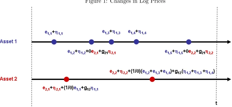
Figure 1 illustrates the mechanism by which tick-time returns are generated in our model. All

distur-bances originating from Asset 1 are colored in blue while all disturdistur-bances originating from Asset 2 are

colored in red. When the first transaction of Asset 1 happens, a value shocke1,1 and a microstructure

disturbanceη1,1are introduced. The first transaction of Asset 2 follows in clock time and since the first

transaction of Asset 1 occurred before it, the return for this transaction is (e2,1+η2,1+_θ1e1,1+g12η1,1),

i.e., the sum of the first value shock of Asset 2,e2,1, the first microstructure disturbance of Asset 2,η2,1,

and a feedback term from the first transaction of Asset 1 whose disturbances aree1,1andη1,1, weighted

by the corresponding feedback impact coefficients 1_θ andg12. In the figure, both log-price processes evolve

until timet. Notice that the third return of Asset 1 contains no feedback term from Asset 2 since there is

no intervening transaction of Asset 2. The second return of Asset 2 includes its own current disturbances

(e2,2, η2,2) as well as six weighted disturbances (e1,2, e1,3, e1,4, η1,2, η1,3 and η1,4) from Asset 1 since

there are three intervening transactions of Asset 1.

At a given clock time t, most of the disturbances of Asset 1 are incorporated into the log price of

Asset 2 and vice-versa. However, there is an end effect. The problem can be easily seen in the figure:

since the fifth transaction of Asset 1 happened after the last transaction of Asset 2 before time t, the

most recent Asset 1 disturbances e1,5 and η1,5 are not incorporated in the log price of Asset 2 at time

t. Eventually, at the next transaction of Asset 2, which will happen after time t, these two disturbances

will be incorporated. But this end effect may be present at any given time t. We will handle this end

effect explicitly in all derivations in the paper.

Our model for the log prices is then given for all non-negative real tby

logP1,t = N_X1(t)

k=1

(e1,k+η1,k) +

N2(t1,N1 (t))

X

k=1

(θe2,k+g21η2,k) (1)

logP2,t = N2(t)

X

k=1

(e2,k+η2,k) +

N1(t2,N2 (t))

X

k=1

(1

θe1,k+g12η1,k) ,

whereti,k is the clock time for thek-th transaction of Asseti, andNi(t) (i= 1,2) are counting processes

which count the total number of transactions of Asset i up to time t. Below, we will impose specific

conditions on {ei,k}, {ηi,k} and Ni(t). Note that (1) implies that logP1,0 = logP2,0 = 0, the same

standardization used in Stock and Watson (1988) and elsewhere. The quantityN2(t1,N1(t)) represents the

total number of transactions of Asset 2 occurring up to the time (t1,N1(t)) of the most recent transaction

of Asset 1. An analogous interpretation holds for the quantityN1(t2,N2(t)).

To exhibit the various components of our model, we rewrite (1) as

logP1,t= ³N1(t)

X

k=1

e1,k+ N2(t)

X

k=1

θe2,k

| {z }

common component

´ +³

N1(t)

X

k=1

η1,k+ N2(t)

X

k=1

g21η2,k

| {z }

microstructure component

´

−

N2(t)

X

k=N2(t1,N1 (t))+1

(θe2,k+g21η2,k)

| {z }

end effect

(2)

logP2,t= ³N1(t)

X

k=1

1

θe1,k+

N2(t)

X

k=1

e2,k

| {z }

common component

´ +³

N1(t)

X

k=1

g12η1,k+ N2(t)

X

k=1

η2,k

| {z }

microstructure component

´

−

N1(t)

X

k=N1(t2,N_{2 (}t))+1

(1

θe1,k+g12η1,k)

| {z }

end effect

.

The common component is a Martingale, and is therefore I(1). We will show that the microstructure

components are I(1 +dη), so these components are less persistent than the common component. The

hence are negligible compared to all other terms. Since both logP1,t and logP2,t areI(1) (see Theorem

1) and the linear combination logP1,t−θlogP2,tisI(1 +dη) as defined in Section III, the log-price series

are cointegrated. (See Theorems 3, 4 and 5.)

Frijns and Schotman (2006) considered a mechanism for generating quotes in tick time which is similar

to the mechanism we describe in Figure 1. However, they condition on durations, whereas we endogenize

them in our model (1). Furthermore, their model implies standard cointegration, with cointegrating

parameter that is known to be 1, and a single value shock component.

Throughout the paper, unless otherwise noted, we will make the following assumptions for our

theo-retical results. The duration processes {τi,k}of Asseti, (i= 1,2), are assumed to possess long memory

with memory parametersdτ1, dτ2 ∈(0,

1

2), in order to reflect the empirically-observed persistence in

dura-tions and the resulting realized volatility. Specifically, the{τi,k}are assumed to satisfy the assumptions

in Theorem 1 of Deo, Hurvich, Soulier and Wang (2007), which are very general and would allow, for

example, the LMSD model of Deo, Hsieh and Hurvich (2006).

We assume that the{ei,k}are mutually independenti.i.d.processes with mean zero and varianceσi,e2 ,

(i= 1,2). We also assume the{ηi,k}to be mutually independent, with zero mean and memory parameter

dηi. For notational convenience, we set dη1 = dη2 = dη in our theoretical results. All theorems will

continue to hold, however, whendη1 anddη2 are distinct, simply by replacingdη withd

∗

η= max(dη1, dη2).

For Theorem 6, which establishes the consistency of the OLS estimator ofθ, we further assume{ei,k}to

beN(0, σ2

i,e).

We assume that {τ1,k} and {τ2,k} are independent of all disturbance series {e1,k}, {e2,k}, {η1,k}

and {η2,k}, which are themselves assumed to be mutually independent. We do not require, however,

that N1(·) and N2(·) be mutually independent, nor do we require that {τ1,k} and {τ2,k} be mutually

independent. This is in keeping with recent literature which suggests that there is feedback between

the counting processes. See, for example, Nijman, Spierdijk and Soest (2004), Bowsher (2007), and the

A

Economic Justification for the Model

Here, we provide some economic rationale for the transaction-level return interactions leading to Model

(1). This supplements our earlier discussion, around Figure 1, on the formal mechanism for price

for-mation. After a brief data analysis affirming the potential usefulness of certain flexibilities of the model,

we compare and contrast the model with a clock-time model proposed by Hasbrouck (1995), and then

propose a transaction-level generalization of Hasbrouck’s definition of the information share of a market.

The model (1) is potentially economically appropriate for pairs of measured prices which are both

affected by the same information shocks (i.e., value shocks), possibly in different ways. Examples include:

buy prices and sell prices of a single stock; prices of two classified stocks (with different voting rights)

from a given company; prices of two different stocks within the same industry; stock and option prices of a

given company; option prices on a given stock with different degrees of maturity or moneyness; corporate

bond prices at different maturities for a given company; Treasury bond prices at different maturities.

The fundamental (value) prices at time t are an accumulation of information shocks. If we ignore

the end effects, these fundamental prices may be thought of as the common components in (2). More

precisely, the fundamental prices may be obtained by setting the microstructure shocks in (1) to zero.

For definiteness, consider the example of buy prices (Asset 1) and sell prices (Asset 2) of a single stock.

Information shocks may be generated on either the buy side or the sell side. According to the model,

each buy transaction generates its own information shock, as does each sell transaction. Furthermore,

these shocks spill over from the side of the market in which they originated to the other side. Clearly,

shocks originating from the sell side of the market cannot be impounded into the buy price until there

is a transaction on the buy side. Similarly, in the absence of information arrivals (transactions) on the

sell side, any string of intervening information shocks from the buy side will render the most recent sell

price stale, until the intervening buy-side shocks are actually impounded into the sell-side price at the

next sell transaction.

the sell side to the buy side are weighted byθ. When θ= 1, shocks spill over from one side to the other

in an identical way, and there is just a single fundamental price, shared by both the buy side and sell

side. In general, as can be seen from (1), the fundamental (log) price for the buy side is an accumulation

of information shocks from both the buy side and the sell side, with the sell-side shocks weighted by θ.

Ignoring end effects, as can be seen from (2), the common component on the buy side is proportional to

the common component on the sell side, and the constant of proportionality isθ.

Analogous interactions take place on the microstructure shocks, such that a microstructure shock

orig-inating on the buy side spills over to the sell side with weightg12 and the opposite spillover occurs with

weight g21. Even in the absence of spillover of the microstructure shocks (g12=g21 = 0), the difference

between the buy price andθtimes the sell price is (except for end effects) an accumulation of

microstruc-ture shocks. It seems in accordance with the economic connotation of the term ”microstrucmicrostruc-ture” that the

microstructure shocks be transitory, i.e., that the aggregate of microstructure shocks be stochastically of

smaller order than the aggregate of fundamental shocks, ast → ∞. This will happen if and only if the

microstructure shocks have a smaller memory parameter than the fundamental shocks (dη <0), as we

assume. Cointegration arises as a consequence of the spillover of the fundamental shocks, together with

the assumption dη <0. The spillover of the fundamental shocks induces the common component while

the assumptiondη <0 ensures that the cointegrating error, arising from microstructure, is less persistent

than the common component.

Two questions that might be raised in the context of Model (1) are whether there are situations

where the two prices are affected by information in different ways, so that the cointegrating parameter

is not equal to 1, and whether it is helpful in practice to allow for fractional cointegration, as opposed

to standard cointegration. To address these questions, we briefly present some results of a preliminary

data analysis. We considered clock-time option bid prices and underlying

best-available-bid prices for IBM on the NYSE at 390 one-minute intervals from 9:30 AM to 4PM on May 31, 2007.

We originally analyzed 74 different options, but removed 5 from consideration since they had either at

least one zero bid price during the day or a constant bid price throughout the day. For the remaining 69

GPH estimator (Geweke and Porter-Hudak, 1983) of the memory parameter of the residuals. The

least-squares regression slopes ranged from −0.21 to 0.39, with a mean of 0.04 and a standard deviation of

0.13. This suggests that information affected the two prices in different ways, for all 69 options. For the

GPH estimators, we used 3900.5_{for the number of frequencies. This results in an approximate standard}

error for the GPH estimator of 0.19. The GPH estimator for the log stock bid price was 1.02. The GPH

estimators for the residuals ranged from 0.05 to 1.14 with a mean of 0.55 and a standard deviation of

0.28. Of the 69 sets of residuals, 62 yielded a GPH estimator less than 1, 54 were less than 0.75, and

42 were less than 0.6. Furthermore, 18 were between 0.4 and 0.6. These results suggest the presence

of cointegration in most cases, and also that the cointegration in some of these cases may be fractional

instead of standard.

It is instructive to compare and contrast our model (1) with the clock-time model of Hasbrouck

(1995), in which a single security is traded on several markets and different market prices share an

identical random-walk component. Suppose, to facilitate comparisons with the bivariate model (1), that

there are two markets. Then for all non-negative integersj, the clock-time log stock prices at timej on

the two different markets are given by Hasbrouck’s model as

logP1,j = logP1,0+

j X

s=1

(ψ1˜e1,s+ψ2e˜2,s) +v1,j (3)

logP2,j = logP2,0+

j X

s=1

(ψ1˜e1,s+ψ2e˜2,s) +v2,j

where logP1,0 and logP2,0 are constants, (˜e1,s,˜e2,s)′ is a zero-mean vector of serially uncorrelated

dis-turbances with covariance matrix Ω, ψ = (ψ1, ψ2) are the weights for ˜e1,s,˜e2,s, and {(v1,j, v2,j)′} is a

zero-mean stationary bivariate time series. The quantity ˜ei,s,(i = 1,2) may be regarded as the

funda-mental shock originating from thei-th market. Hasbrouck (1995) estimated the model on data using a

one-second sampling interval.

Both Models (1) and (3) induce a common component, and cointegration. Both have spillover of

the fundamental shocks from one market to the other. In Model (3) the spillover is the same in both

directions so the common components are identical and the cointegrating parameter is 1, in contrast to

isI(0), while in Model (1) the cointegrating error is allowed to beI(1 +dη) for anydη with−1≤dη <0.

In Model (3) the contemporaneous correlation between the fundamental shocks originating from the

two markets is allowed to be nonzero, (i.e., Ω is allowed to be non-diagonal), whereas in Model (1) the two

fundamental shock series are assumed to be independent. Note, however, that in the transaction-level

model (1), thekth_{transactions of the two assets will (almost surely) occur at different clock times, so any}

correlation between the two fundamental shockse1,k ande2,kwould fail to be contemporaneous in clock

time. This provides one motivation for our assumption that{e1,k}and{e2,k}are mutually independent.

An economic motivation for this assumption stems from the following remarks of Hasbrouck (1995, p.

1183): ”In practice, market prices usually change sequentially: a new price is posted in one market, and

then the other markets respond. If the observation interval is so long that the sequencing cannot be

determined, however, the initial change and the response will appear to be contemporaneous. Therefore,

one obvious way of minimizing the correlation is to shorten the interval of observation.” Since Model (1)

is defined in continuous time, the interval of observation is effectively zero, so at least under the idealized

assumptions that there are no truly simultaneous transactions on the two markets and that the time

stamps for the transactions are exact, the assumption of mutual independence would be economically

reasonable.

In the remainder of this subsection, we discuss the information share, originally defined in

Has-brouck (1995) to measure how market information that drives stock prices is distributed across

dif-ferent exchanges. Hasbrouck (1995) defined the information share of market i based on Model (3) as

Si = (ψi2Ωii)/(ψΩψ′), which is the proportional contribution from market i to the total fundamental

innovation variance. Only the random-walk component is used in constructing the information share

since this is the only permanent component. As discussed in Hasbrouck (1995), the fact that Ω may not

be diagonal has the consequence that only a bound for the information share can be estimated. Below,

we propose a transaction-level generalization of the concept of information share based on Model (1),

which is directly estimable due to our assumption of mutual independence of the transaction-level

funda-mental disturbance series. The information share proposed in Hasbrouck (1995) measures how the price

how the price-driving information of a security is distributed between buy versus sell trades in a market.

The ideas are similar. Indeed, as mentioned in Hasbrouck (1995), his model can be extended to model

bid and ask prices dynamics. Nevertheless, as discussed above, our model ultimately is a tick-level model

which is different from existing clock-time models, including that in Hasbrouck (1995).

For Model (1), we define the information share as follows: for a given clock-time sampling interval

∆t, the information share of Assetiis given by

S1,C =

var³ PN1(j∆t)

k=N1((j−1)∆t)+1e1,k

´

var³ PN1(j∆t)

k=N1((j−1)∆t)+1e1,k+θ

PN2(j∆t)

k=N2((j−1)∆t)+1e2,k

´ = λ1σ

2 1,e

λ1σ21,e+θ2λ2σ22,e

(4)

S2,C=

θ2_λ 2σ22,e

λ1σ21,e+θ2λ2σ22,e

,

where λi is the intensity of the counting process Ni(·) (see Daley and Vere-Jones 2003), and represents

the intensity of trading (level of market activity) of Asset i. The ultimate expressions for Si,C do not

depend on the sampling interval ∆t. Note that only the common component in (2) is used to evaluate the

information share, as was also done by Hasbrouck (1995). Asλ1/λ2→ ∞,S1,C approaches one andS2,C

approaches zero. This is consistent with general intuition: an actively-traded security should reveal more

information than a thinly-traded one. Indeed, Hasbrouck (1995) found that, for the 30 Dow-Jones stocks,

the preponderance of the price discovery takes place at the NYSE and the majority of the transactions

occurred on the NYSE. The information shareSi,C can be estimated using the transaction-level method

of moments as described in section VIII. We exhibit estimates of Si,C computed from transaction-level

data in Section XI.

III

Conditions on the Microstructure Noise for Fractional and

Standard Cointegration

We consider three types of cointegration: weak fractional, strong fractional and standard cointegration.

The weak fractional cointegration case corresponds todη ∈(−1₂,0). In this case, we will require the

following condition, stated for a generic process{ηk}.

Condition A _{Fordη ∈(−}1

2,0),{ηk} is a weakly stationary zero-mean process with memory parameter

dη in the sense that the spectral density f(λ)satisfies

f(λ) = ˜σ2C∗λ−2dη_{(1 +O(λ}β_{)) as λ} →0+

for someβ with0< β≤2, whereσ˜2_{>0 andC}∗_{= (d}

η+1₂)Γ(2dη+ 1) sin((dη+1₂)π)/π >0.

Condition A, which was originally used in a semiparametric context by Robinson (1995), is very

general, since it only specifies the behavior of the spectral density in a neighborhood of zero frequency.

The condition is satisfied by all parametric long-memory models that we have seen in the literature,

including the ARFIMA(p, dη, q) model withp≥0,q≥0 anddη∈(−1₂,0). In the ARFIMA case,β= 2.

Condition A also allows the possibility for seasonal long memory, i.e., poles or zeros of f(λ) at nonzero

frequencies.

The strong fractional cointegration case corresponds to dη∈(−1,−1₂). For this case, we assume

Condition B _{Fordη∈(−1,−}1

2),ηk =ϕk−ϕk−1,k= 1,2, . . .whereϕ0= 0and{ϕk}∞k=1is a zero-mean

weakly-stationary long-memory process with memory parameterdϕ=dη+ 1∈(0,1₂)in the sense that its

autocovariances satisfy

cov(ϕk, ϕk+j) =Kj2dϕ−1+O(j2dϕ−3) , j≥1 (5)

whereK >0.

By Theorem 1 of Lieberman and Phillips (2006), any stationary, invertible ARFIMA(p, dϕ, q) process

withdϕ∈(0,1₂) has autocovariances satisfying (5), withK= 2f∗(0)Γ(1−2dϕ) sin(πdϕ), wheref∗(0) is

the spectral density of the ARMA component of the model at zero frequency.

The standard cointegration case corresponds to dη =−1. In this case we assume

Condition C _{If dη =−1, {ηk}}∞

weakly stationary with zero mean and has autocovariance sequence{cξ,r}∞r=0 wherecξ,r=E(ξk+rξk)with

exponential decay,|cξ,r| ≤Aξe−Kξr for allr≥0, where Aξ andKξ are positive constants.

The assumptions on {ξk} in Condition C above are satisfied by all stationary, invertible ARMA

models.

IV

Long-Term Martingale-Type Properties of the Log Prices

In this section, we present the properties of the log-price series generated by Model (1). Define λi =

1/E0_{(τi,k), where E}0 _{denotes expectation under the Palm distribution (See Deo, Hurvich, Soulier and}

Wang 2007 for discussions about the Palm probability measure), i.e., the distribution under which the

{τi,k}, (i = 1,2) are stationary. The following two theorems show that the log-price series in Model

(1) have asymptotic variances that scale like t as t → ∞, as would happen for a Martingale, and that

their discretized differences are asymptotically uncorrelated as the sampling interval increases, as would

happen for a Martingale difference series.

Theorem 1 _{For the log-price series in Model (1),}

var(logPi,t)∼Cit, i= 1,2

ast→ ∞, whereC1= (σ12,eλ1+θ2σ22,eλ2)andC2= (σ22,eλ2+_θ12σ21,eλ1).

For a given sampling interval (equally-spaced clock-time period) ∆t, the returns (changes in log price)

for Asset 1 and 2 corresponding to Model (1) are

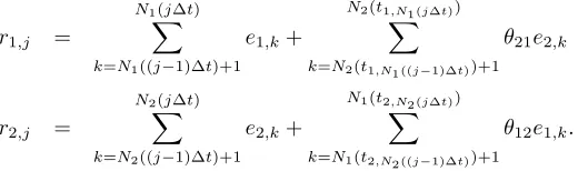
r1,j =

N1(j∆t)

X

k=N1((j−1)∆t)+1

(e1,k+η1,k) +

N2(t1,N1 (j∆t))

X

k=N2(t1,N1 ((j−1)∆t))+1

(θe2,k+g21η2,k) (6)

r2,j =

N2(j∆t)

X

k=N2((j−1)∆t)+1

(e2,k+η2,k) +

N1(t2,N_{2 (}j∆t))

X

k=N1(t2,N_{2 ((}j−1)∆t))+1

(1

Theorem 2 _{For any fixed integer k >0, the lag-k autocorrelation of {ri,j}}∞_{j=1, i = 1,2, tends to 0 as}

∆t→ ∞.

V

Properties of the Cointegrating Error

We show that Model (1) implies a cointegrating relationship between the two series, treating the weak

and strong fractional as well as standard cointegration cases separately.

Theorem 3 _{Under Model (1) with dη ∈ (−}1

2,0), the memory parameter of the linear combination

(logP1,t−θlogP2,t)is (1 +dη)∈(12,1), that is,

var(logP1,t−θlogP2,t)∼C t2dη+1

ast→ ∞, whereC >0. In this sense,logP1,t andlogP2,t are weakly fractionally cointegrated.

Next, we investigate the standard cointegration case. It is important to note that, unlike in Theorem

3, where we measure the strength of cointegration using the asymptotic behavior of the variance of the

cointegrating errors var(logP1,t−θlogP2,t), we need a different measure here since logP1,t−θlogP2,t

is stationary and its variance is constant for allt. Instead, we consider the asymptotic covariance of the

cointegrating errors

cov(logP1,t−θlogP2,t,logP1,t+j−θlogP2,t+j)

asj→ ∞. We taketandj here to be positive integers,i.e., we sample the log-price series using ∆t= 1,

without loss of generality.

Theorem 4 _{Under Model (1) with dη ∈ (−1,−}1

2), the memory parameter of the cointegrating error

(logP1,t−θlogP2,t)is (1 +dη)∈(0,1₂), that is, for any fixed t >0,

cov³logP1,t−θlogP2,t, logP1,t+j−θlogP2,t+j ´

∼j2(1+dη)−1_[C

1P r{N1(t)>0}+C2P r{N2(t)>0}]

We say that a sequence{aj}hasnearly-exponential decay ifaj/j−α→0 asj → ∞for allα >0. We

say that a time series hasshort memory if its autocovariances have nearly-exponential decay.

Theorem 5 _{Under Model (1), with dη = −1, the cointegrating error (logP1,t −θlogP2,t) has short}

memory. In this sense,logP1,t andlogP2,t are cointegrated.

VI

Least-Squares Estimation of the Cointegrating Parameter

Assume that the log-price series are observed at integer multiples of ∆t. The proposed model (1) becomes

(with a minor abuse of notation)

logP1,j =

N1_X(j∆t)

k=1

(e1,k+η1,k) +

N2(t1,N₁₍j∆t))

X

k=1

(θe2,k+g21η2,k) (7)

logP2,j =

N2_X(j∆t)

k=1

(e2,k+η2,k) +

N1(t2,N2(j∆t))

X

k=1

(1

θe1,k+g12η1,k) .

We show that the cointegrating parameterθcan be consistently estimated by OLS regression.

Theorem 6 _{For the discretely-sampled log-price series in (7) with normally distributed value shocks}

{e1,k},{e2,k}, the cointegrating parameterθcan be consistently estimated byθˆ, the ordinary least squares

estimator obtained by regressing{logP1,j}nj=1on{logP2,j}nj=1without intercept. For allδ >0, asn→ ∞,

we have

Case I: dη∈(−1₂,0)

n−dη−δ_{(ˆθ−θ)−→}p _0,

Case II: dη ∈(−1,−1₂)

n12−δ(ˆθ−θ)−→p 0,

Case III: dη =−1

In the weak fractional cointegration case dη ∈ (−1₂,0), the rate of convergence of ˆθ improves as dη

decreases. In the standard cointegration case where dη = −1, the rate is arbitrarily close to n. The

n-consistency (super-consistency) of the OLS estimator of the cointegrating parameter in the standard

cointegration case has been shown for time series in discrete clock time that are linear with respect to

a strong-mixing or i.i.d. sequence by Phillips and Durlauf (1986) and Stock (1987). We are currently

unable to derive the asymptotic distribution of the OLS estimator of the cointegrating parameter in the

standard cointegration case for our model, as we cannot rely on the strong-mixing condition on returns.

This condition would not be expected to hold in the case of LMSD durations, since these are not

strong-mixing in tick time. In the strong fractional cointegration casedη ∈(−1,−1₂), though we have established

a rate ofn1/2−δ_{, simulations in Section X indicate that the actual rate is faster, atn}−dη−δ_{, in keeping}

with the rates obtained in the weak fractional and standard cointegration cases.

VII

A Tick-level Cointegrating Parameter Estimator

We propose a transaction-level estimator, ˜θ, for the cointegrating parameterθ in this section. It may be

argued that the OLS estimator ˆθdiscussed in Section VI is not optimal since it is constructed based on

discretized log-prices, and therefore only uses partial information. Here we propose a tick-level estimator,

˜

θ, that utilizes the full tick-level price series, logP1,t, logP2,t fort∈[0, T].

Specifically, letN(T) =N1(T) +N2(T) be the pooled counting process of transactions for both Asset

1 and Asset 2 in the time interval (0, T], and denote by {t⋆ k}

N(T)

k=1 the transaction times for the pooled

process. The proposed estimator is

˜

θ =

RT

0 logP1,t·logP2,tdt

RT

0 logP 2 2,tdt

(8)

=

PN(T)−1

j=1

h

logP1,N1(t⋆j)·logP2,N2(t⋆j)

i

·(t⋆

j+1−t⋆j) + h

logP1,N1(T)·logP2,N2(T)

i

·(T−t⋆ N(T))

PN2(T)−1

j=1 logP22,j·τ2,j+1+ logP₂2_,N2(T)·(T−t2,N2(T))

,

where the numerator is a summation over all transactions, adding up the product of the most recent

denominator of ˜θ has the same structure except that the product is now of Asset 2 log-prices with

themselves.

We do not derive asymptotic properties of the estimator ˜θ. Nevertheless, the simulation study in

Section X indicates that the tick-level estimator ˜θ may outperform the OLS estimator ˆθ, having smaller

bias, variance and Root-Mean-Squared-Error (RMSE), particularly if the sampling interval ∆t for ˆθ is

large.

VIII

Method of Moments Parameter Estimation

In Section XIV, we will propose a transaction-level parameter estimation procedure for model (1) using

the method of moments, based on logP1,t, logP2,t fort ∈[0, T]. We will make specific assumptions for

the sake of definiteness, though most of these assumptions could be relaxed. Specifically, we will assume

Gaussian white noise for the value shocks, a Gaussian ARFIMA(1, dη,0) process for the microstructure

noise whendη∈(−1₂,0), while we will assume that the microstructure noise is the difference of a Gaussian

ARFIMA(1, dη+ 1,0) process with the initial value set to zero when dη ∈ (−1,−1₂). In the standard

cointegration casedη=−1, we will assume that the microstructure noise is the difference of a Gaussian

AR(1) process with initial value set to zero.

The method-of-moments estimator ˆΘ = (ˆσ2

1,e,σˆ22,e,ˆσ12,η,ˆσ22,η,gˆ21,ˆg12,dˆη1,dˆη2,αˆ1,αˆ2) is obtained as

the solution to a system of ten equations, as described in Section XIV, where we will also establish the

following theorem on consistency of the estimator.

Theorem 7 _{The method-of-moments estimatorΘ}ˆ _{is consistent, i.e.}

ˆ

Θ→p Θ, asT → ∞

whereΘ = (σ2

1,e, σ22,e, σ12,η, σ22,η, g21, g12, dη1, dη2, α1, α2).

propose an alternative ad hoc estimator ˜Θ in Section XIV. We evaluate the performance of ˜Θ in a

simulation study in Section X.

IX

Model Specification Test

In this section, we propose a specification test for our model (1), based on Theorem 6. The idea is that,

according to Theorem 6, if the model (1) is correctly specified, then the OLS estimator is consistent for

any particular sampling interval ∆t. Suppose we choose two sampling intervals, ∆t1and ∆t2, and denote

the corresponding OLS estimators by ˆθ∆t1_{and ˆθ}∆t2_{. Since both estimators are consistent, their difference}

must converge in probability to zero. Thus, we propose a specification test to test whether this difference

is significantly different from zero. The test is semiparametric, in that model (1) makes no parametric

assumptions on either the durations or the microstructure noise.

To implement the test, we divide the entire time span, say one year, intoKnonoverlapping subperiods,

e.g., divide the data set into months. Within subperiodk,(k= 1, . . . , K), we sample every ∆t1to obtain

a bivariate log-price series{logP∆t1

1,j,k,logP

∆t1

2,j,k}, where logP

∆t1

1,j,k is thej-th sampled Asset 1 log-price in the subperiodkusing sampling interval ∆t1and similarly for logP2∆,j,kt1. Based on these, we obtain an OLS

cointegrating parameter estimate ˆθ∆t1

k , and similarly we sample every ∆t2to obtain{logP1∆,j,kt2,logP

∆t2

2,j,k} and then obtain ˆθ∆t2

k . Repeating the procedure through allKsubperiods, we obtain sequences{θˆ

∆t1

k }Kk=1

and{θˆ∆t2

k }Kk=1. The test statistic is proposed to be

ˆ

δ12=

sample mean of{δˆ12,k} q

1

K·sample variance of{δˆ12,k}

where ˆδ12,k= ˆθk∆t2−θˆ

∆t1

k ,(k= 1, . . . , K). The distribution of the test statistic under the null hypothesis that all model assumptions are correctly specified is unknown. However, the critical value for the test

as well as the corresponding distribution of the test statistic can be simulated under the null hypothesis,

based on the estimated parameter values.

specified. Similarly as discussed in Hausman (1978), one sufficient requirement is that the two estimators, ˆ

θ∆t1 _{and ˆθ}∆t2_{, have different probability limits under the alternative, in order for the specification test}

to be consistent.

In Section X, we first investigate the simulation-based distributions of the test statistics for

empirically-relevant parameter values, then compute critical values for the specification test on the empirical example,

Tiffany (TIF), which are later used in the data analysis in section XI.

X

Simulations

A

The Estimation of the Cointegrating Parameter:

θ

ˆ

_and

θ

˜

We study the performance of ˆθ as well as ˜θin a simulation study carried out as follows.

First, we simulate two mutually independent duration process{τi,k} for Asseti= 1,2. Note that for

simplicity we take the two duration processes to be mutually independent, although this is not required

by our theoretical results. Each duration process follows the Long Memory Stochastic Duration (LMSD)

model,

τi,k=ehi,kǫi,k

where the{ǫi,k}arei.i.d.positive random variables with all moments finite, and the{hi,k}are a Gaussian

long-memory series with zero mean and common memory parameter dτ. Based on empirical work in

Deo, Hsieh and Hurvich (2006), we choosedτ1 =dτ2 = 0.45. Here, we assume that the{ǫi,k} follow an

exponential distribution with unit mean. We simulated the{hi,k} from a Gaussian ARFIMA(0,dτ, 0)

model, with innovation variances chosen so that the mean of the log durations matches those observed

in the Tiffany series used in Section XI. Using the simulated durations{τi,k},i= 1,2, we obtained the

corresponding counting processes {Ni(t)}, using ti,1 = Uniform[0, τi,1]. This ensures that the counting

Next, we generate mutually independent disturbance series {e1,k},{e2,k},{η1,k} and {η1,k}. Here,

{ei,k}, i = 1,2, are i.i.d. Gaussian with zero means. For simplicity, the memory parameters of the

microstructure noise series are assumed to be the same: dη1 = dη2 = dη. When dη ∈ (−

1

2,0), the

{ηi,k} are given by ARFIMA(1, dη, 0). Whendη ∈(−1,−1₂), {ηi,k} are simulated as the differences of

ARFIMA(1, dη + 1, 0); and when dη =−1,{ηi,k} are simulated as the differences of two independent

zero-mean Gaussian AR(1) series {ξi,k}. The disturbance variances were var(ei,k) = 4×10−6 and

var(ηi,k) = 1×10−6 _{fori= 1,2. Also, we setg}

21=g12= 1. We selected these particular values as they

are close to the corresponding parameter estimates based on several stocks that we analyzed empirically.

We then constructed the log-price series{logPi,j}nj=1, i= 1,2 from (1), using a fixed sampling interval

∆t. We calculated the estimated cointegrating parameter ˆθby regressing{logP1,j}jn=1 on{logP2,j}nj=1,

using ordinary least squares without intercept. The tick-level estimator, ˜θis constructed according to (8)

using the entire tick-level price series.

In the study, we fixed the cointegrating parameter at θ = 1. We considered various values of the

parameters ∆tand the sample sizen. We think of time as being measured in seconds, so that ∆t= 300

corresponds to observing the price series every 5 minutes, and in this case n = 390 would correspond

to one week of data. (Each day, there are 6.5 trading hours so sampling every 5 minutes yields 78

observations per day). For each parameter configuration, we generated 1000 realizations of the log-price

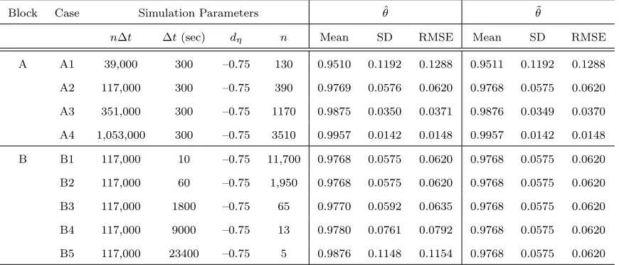
series. The results are summarized in Table 1.

As the sample size nincreases, the bias, the standard deviation and the Root-Mean-Squared Error

(RMSE) of ˆθdecrease, as seen in Block A. This is consistent with Theorem 6. We only report results for

dη=−0.75, however we found similar patterns for dη =−0.25,−1.

In A2 together with Block B, we fix the total time spanT =n∆t, while varying the sampling interval

∆t and n. For this specific set of empirically-relevant parameter values, the impact of increasing ∆t is

not obvious until ∆t = 9000, which corresponds to the commonly-used sampling frequency of one day.

Both the standard deviation and the RMSE deteriorate as ∆t grows. We found the same pattern for

Table 1: Simulation Results on the Estimation of the Cointegrating Parameter

Block Case Simulation Parameters θˆ θ˜

n∆t ∆t(sec) dη n Mean SD RMSE Mean SD RMSE

A A1 39,000 300 –0.75 130 0.9510 0.1192 0.1288 0.9511 0.1192 0.1288 A2 117,000 300 –0.75 390 0.9769 0.0576 0.0620 0.9768 0.0575 0.0620 A3 351,000 300 –0.75 1170 0.9875 0.0350 0.0371 0.9876 0.0349 0.0370 A4 1,053,000 300 –0.75 3510 0.9957 0.0142 0.0148 0.9957 0.0142 0.0148 B B1 117,000 10 –0.75 11,700 0.9768 0.0575 0.0620 0.9768 0.0575 0.0620 B2 117,000 60 –0.75 1,950 0.9768 0.0575 0.0620 0.9768 0.0575 0.0620 B3 117,000 1800 –0.75 65 0.9770 0.0592 0.0635 0.9768 0.0575 0.0620 B4 117,000 9000 –0.75 13 0.9780 0.0761 0.0792 0.9768 0.0575 0.0620 B5 117,000 23400 –0.75 5 0.9876 0.1148 0.1154 0.9768 0.0575 0.0620

ˆ

θ decreases as the sampling interval ∆t increases, possibly due to the fact that the end effect is not as

important when ∆tis large. Finally, in terms of RMSE, ˜θperforms no worse than ˆθ, and performs much

better than ˆθ when ∆t is large.

We also performed simulations related to the convergence rate of ˆθ. In Theorem 6, when dη ∈

(−1,−1

2), the convergence rate is shown to be arbitrarily close to

√_{n and does not depend on dη.}

However, simulations indicate a faster rate in this strong fractional cointegration case. For example,

when dη =−0.75, we simulated the log price series in discrete clock-time using sample sizes nranging

from 1,000 to 20,000 with an equally-spaced increment of 800. The variance of ˆθ for each value of n

was obtained based on 1,000 realizations. The estimated convergence rate of ˆθ is n0.78_{, obtained from}

the estimated slope in a log-log plot of these simulated variances versus the corresponding sample sizes.

We ran similar simulations for other values of dη. Based on these, we conjecture that the actual rate

of convergence for ˆθ isn−dη−δ_{, in keeping with the rates obtained in the weak fractional and standard}

B

The performance of

Θ

˜

We carried out a simulation study to evaluate the performance of the ad hoc estimator ˜Θ of Θ discussed

in Section XIV. The parameter values weredτ1 =dτ2 = 0.45, dη1 =dη2 =−0.25,−0.75,−1.00, θ = 1,

var(ei,k) = 4×10−6_{,(i= 1,2), var(ηi,k) = 1×10}−6_{,(i= 1,2), g}

12=g21= 1, andα1=α2 =−0.5. The

{hi,k} were simulated as in Section X.

We simulated log prices in model (1) for a clock-time span of n∆t, with n = 1716 and ∆t = 300

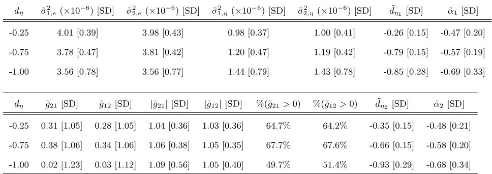
seconds (corresponding to a clock-time span of one month). The results, given in Table 2, are averages

based on the 1000 realizations, after excluding those realizations that give negative estimates for ˜g2 21 or

˜

g2

12 which happen about 15% of the time. The estimates for both σ2i,e,(i= 1,2) and σi,η2 ,(i= 1,2) are

Table 2: Parameter Estimation using ˜Θ

dη σ˜21,e(×10−6) [SD] σ˜22,e(×10−6) [SD] σ˜12,η(×10−6) [SD] σ˜22,η (×10−6) [SD] d˜η1 [SD] α˜1 [SD]

-0.25 4.01 [0.39] 3.98 [0.43] 0.98 [0.37] 1.00 [0.41] -0.26 [0.15] -0.47 [0.20]

-0.75 3.78 [0.47] 3.81 [0.42] 1.20 [0.47] 1.19 [0.42] -0.79 [0.15] -0.57 [0.19]

-1.00 3.56 [0.78] 3.56 [0.77] 1.44 [0.79] 1.43 [0.78] -0.85 [0.28] -0.69 [0.33]

dη g˜21[SD] ˜g12 [SD] |g˜21|[SD] |g˜12|[SD] %(˜g21>0) %(˜g12>0) d˜η2 [SD] α˜2 [SD]

-0.25 0.31 [1.05] 0.28 [1.05] 1.04 [0.36] 1.03 [0.36] 64.7% 64.2% -0.35 [0.15] -0.48 [0.21]

-0.75 0.38 [1.06] 0.34 [1.06] 1.06 [0.38] 1.05 [0.35] 67.7% 67.6% -0.66 [0.15] -0.58 [0.20]

-1.00 0.02 [1.23] 0.03 [1.12] 1.09 [0.56] 1.05 [0.40] 49.7% 51.4% -0.93 [0.29] -0.68 [0.34]

reasonably well-behaved. The magnitudes ofg21 and g12 are also well estimated, but the signs are not.

This is due to the fact that these signs are determined based on certain five-trade sequences (instead of

certain three-trade sequences to estimate the magnitudes) that occur relatively infrequently in the data

(see Section XIV in the Appendix for details). Histograms of ˜g21 or ˜g12 show a bimodal distribution,

C

Specification Test

We perform a simulation study on the specification test proposed in Section IX. Two sets of

empirically-relevant parameter values are used to investigate the simulation-based distribution of the test statistic

ˆ

δ.

We choose empirically-relevant parameter values to investigate the simulation-based distribution of

the test statistic ˆδ. Specifically, we selected four sampling intervals ∆t1= 60, ∆t2= 300, ∆t3= 600 and

∆t4 = 1800 seconds, respectively. The entire time span is set to be 100 trading days, which is divided

into 25 subperiods with 4 trading days each. Other model parameter values are: dη = dη1 = dη2 =

−0.25,−0.75,dτ1 =dτ2 = 0.45. Results are based on 1000 realizations.

Six test-statistic distributions are generated for each pair of sampling intervals. For example, for the

pair ∆t1, ∆t2, we obtain a test statistic

ˆ

δ12,m=

sample mean of{θˆ∆t2

k,m−θˆ

∆t1

k,m} q

1

25·sample variance of{θˆ ∆t2

k,m−θˆ

∆t1

k,m}

for realization m based on {θˆ∆t1

k,m}25k=1 and {θˆ ∆t2

k,m}25k=1. Overall, we have {ˆδ12,m}1000m=1, which form the

simulation-based empirical distribution of the test statistic ˆδ12. This distribution can be used to generate

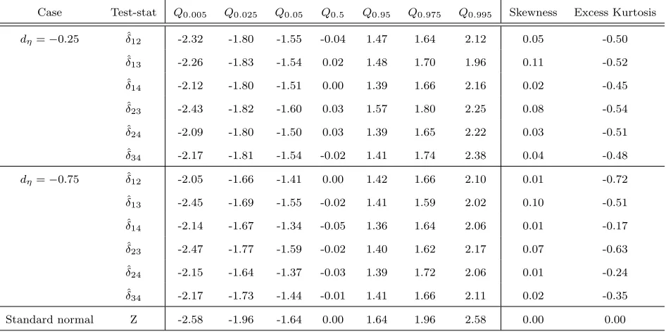
critical values or compute empirical p-values. In Table 3, we summarize the quantiles of these

empir-ical distributions, where Qq represents the q-th quantile. For each distribution, the null hypothesis of

normality is rejected at a nominal size of 1% based on the Kolmogorov-Smirnov Goodness-of-Fit Test.

XI

Data Analysis

In this section, we focus on analyzing the buy prices{P1,t} and sell prices{P2,t}of a single stock. The

stock we consider is Tiffany Co. (ticker: TIF). The data were obtained from the TAQ database of WRDS.

We considered daily transactions between 9:30 AM and 4:00 PM. Overnight durations and returns are

Table 3: Summary Statistics of the Simulation-based Empirical Distributions

Case Test-stat Q0.005 Q0.025 Q0.05 Q0.5 Q0.95 Q0.975 Q0.995 Skewness Excess Kurtosis dη=−0.25 ˆδ12 -2.32 -1.80 -1.55 -0.04 1.47 1.64 2.12 0.05 -0.50

ˆ

δ13 -2.26 -1.83 -1.54 0.02 1.48 1.70 1.96 0.11 -0.52

ˆ

δ14 -2.12 -1.80 -1.51 0.00 1.39 1.66 2.16 0.02 -0.45

ˆ

δ23 -2.43 -1.82 -1.60 0.03 1.57 1.80 2.25 0.08 -0.54

ˆ

δ24 -2.09 -1.80 -1.50 0.03 1.39 1.65 2.22 0.03 -0.51

ˆ

δ34 -2.17 -1.81 -1.54 -0.02 1.41 1.74 2.38 0.04 -0.48 dη=−0.75 ˆδ12 -2.05 -1.66 -1.41 0.00 1.42 1.66 2.10 0.01 -0.72

ˆ

δ13 -2.45 -1.69 -1.55 -0.02 1.41 1.59 2.02 0.10 -0.51

ˆ

δ14 -2.14 -1.67 -1.34 -0.05 1.36 1.64 2.06 0.01 -0.17

ˆ

δ23 -2.47 -1.77 -1.59 -0.02 1.40 1.62 2.17 0.07 -0.63

ˆ

δ24 -2.15 -1.64 -1.37 -0.03 1.39 1.72 2.06 0.01 -0.24

ˆ

δ34 -2.17 -1.73 -1.44 -0.01 1.41 1.66 2.11 0.02 -0.35

Standard normal Z -2.58 -1.96 -1.64 0.00 1.64 1.96 2.58 0.00 0.00

25, 2000 to July 20, 2000, comprising 124 trading days.

We follow Lee and Ready (1991) to classify individual trades. If the transaction price is higher than

the prior bid-ask midpoint, the current trade is labeled as a buy order. If the transaction price is lower,

it is labeled as a sell order. If the transaction price is exactly the same as the prior bid-ask midpoint,

the tick test (described in Lee and Ready 1991) is used to decide whether it should be classified as a buy

or sell order. Lee and Ready (1991) found that the accuracy of their method is at least 85%. Using this

method, we found 26,103 buy trades and 32,812 sell trades during the period of study.

We first verify that a strong cointegrating relationship exists between buy and sell prices of TIF. The

results are given in Table 4. We estimated the memory parameters of the log buy prices and log sell

prices as 1 plus the GPH estimator (see Geweke and Porter-Hudak, 1983) of the memory parameter of

the differences. We estimated the memory parameter of the cointegrating error using a GPH estimator

of ∆t. Note that the memory parameter of the cointegrating error is 1 + max(dη1, dη2). The number of

frequencies used in the log periodogram regressions was n0.5 _{As expected, the estimated cointegrating}

parameter is close to 1. Evidence of strong cointegration is observed. Furthermore, there is some evidence

that the cointegration is fractional, not standard.

Table 4: Buy and Sell Prices of TIF

∆t(sec) n estimate ofθ dˆbuy-price[SE] dˆsell-price[SE] dˆcoint-error[SE]

1800 1612 θˆ= 0.998040 1.0124 [0.0484] 1.0105 [0.0484] 0.2328 [0.0484]

600 4836 θˆ= 0.998046 1.0223 [0.0330] 1.0208 [0.0330] 0.1312 [0.0330]

300 9672 θˆ= 0.998042 0.9906 [0.0259] 0.9914 [0.0259] 0.1068 [0.0259]

− − θ˜= 1.001678 − − −

Next, using the ad hoc estimator ˜Θ, we estimated the model parameters for three clock-time

subperi-ods, as well as the entire period. Period one spans day 1 to day 25, during which the stock price declined

by roughly 25%. Period two spans day 41 to day 70, where the price was relatively stable. Period three

spans day 90 to day 124, during which the stock price raised by approximately 25%. The results are

given in Table 5. The tick-time stock prices are plotted in Figure 2.

Table 5: Method of Moments Parameter Estimates of TIF

Period Type # of trades ˜σ2

i,e(×10−6) σ˜i,η2 (×10−6)

1: trading day 1 to 25 Buy 5,852 3.01 3.38

Sell 6,875 3.05 1.93

2: trading day 41 to 70 Buy 5,360 6.22 0.72

Sell 7,688 4.08 0.83

3: trading day 90 to 124 Buy 6,896 3.50 1.18

Sell 8,827 2.00 2.66

entire period Buy 26,103 4.67 1.26

Figure 2: TIF Transaction-level Stock Price

Based on the results in Table 5, we report the following findings:

1) The microstructure noise variance estimates (˜σ2

i,η) are smaller for subperiod two (during which the stock prices vary substantially but do not show a clear trend), than for subperiods one and three (during

which the price showed decreasing and increasing trends, respectively).

2) The value-shock variance estimates (˜σ2

i,e) show an opposite pattern, i.e., larger in subperiod two but smaller in subperiods one and three.

3)Comparing ˜σ2

i,e and ˜σi,η2 , the variability of the value shocks usually dominates exceeds that of the microstructure shocks. Indeed, ˜σ2

i,e is greater than ˜σ2i,η for both buy and sell trades in the entire period.

As for the microstructure noise feedback coefficient estimates, ˜g21 and ˜g12, their magnitudes are

generally around 1, but the signs vary in different subperiods. In some subperiods, the estimates of ˜g2 21

or ˜g2

12are negative, thus we set the corresponding ˜g21or ˜g12to be zero. In general, no systematic pattern

is observed for ˜g21 and ˜g12 and their values are not reported in Table 5. We stress, however, that the

simulation study in Section X showed thatg21andg12are harder to estimate than the other parameters.

market-maker executes buy and sell orders that arrive randomly, with the arrival rate being determined by the

quoted bid and ask prices, so as to maximize his expected profit per unit time, under the constraint that

his inventory position will not exceed a long and a short positions – L and S respectively. (The analysis

applies to traders who act as market makers, that is, quote buying and selling prices and benefit from

trading at these prices, rather taking a long-run position in the stock, based on some information.) The

market maker sets the pair of bid-ask prices to adjust his inventory, and his policy results in having a

preferred inventory position towards which he reverts. The bid-ask spread is minimized at this preferred

position while it increases as the inventory diverges from the preferred level. This policy applies when

there is no change in information about the security’s value, in which case prices show no clear trend,

hovering within a range. Amihud and Mendelson (1982, pp. 56-58) analyze a situation of a change

in information about the security’s value, unknown to the market maker. At first, the market maker

maintains the schedule of bid and ask prices that applies to the old valuation, but given the value change,

his inventory will deviate from the preferred position and the bid-ask spread will widen. (For example,

if the value is lower, the market maker will accumulate a large long position, quoted prices will decline

and the bid-ask spread will widen.) After having realized that the value has changed, the market maker

shifts his schedule of quoted bid and ask prices and the bid-ask spread reverts to a normal, narrower

range. Applying this analysis to the data, subperiods 1 and 3 show a major shift in the security value,

reflected in the trend in price. By Amihud and Mendelson (1982), a period of shift in value is associated

with wider bid-ask spread. In subperiod 2, when prices vary but do not show a clear trend, the bid-ask

spread should be narrower.

A narrower bid-ask spread (a smaller spread magnitude) indicates a smaller microstructure noise

variance (see Amihud and Mendelson 1987, pp. 536, 547), i.e. smallerσ2

η,i in Model (1). Indeed, we found that the estimated microstructure noise variances are smaller when price fluctuates without a clear

trend (subperiod 2) and larger otherwise (subperiods 1 and 3). Unfortunately, it is not possible to test

the significance of the change in microstructure noise variances across the three subperiods since the

estimates are not independent.

Specifically, here we focus on the price discovery of a single stock, e.g., TIF, during different market

environments. To estimate the information share, estimates for the trading intensities λ1, λ2, and the

value-shock variances σ2

1,e, σ22,e are required. To estimate λi,(i = 1,2), we use the total number of transactions divided by the total period of observation for asset i. We estimate σ2

1,e and σ22,e by the method of moments as discussed in section VIII. We compute the information share estimates for each

of three clock-time subperiods based on results in Table 5. Results are summarized in Table 6.

Table 6: Information Shares (S) of Buy and Sell Price of TIF

Period S˜buy S˜sell ( ˜Sbuy−S˜sell)

1: Trading day 1 to 25 45.7% 54.3% -8.6%

2: Trading day 41 to 70 51.5% 48.5% 3.0%

3: Trading day 90 to 124 57.5% 42.3% 15.2%

Entire Period 52.6% 47.4% 5.2%

For period two, the information shares are approximately equally divided between buys and sells. For

period one when the stock price declines dramatically, the sell trades possess more information than buy

trades. By contrast, during period three when price is rising, the buy trades have more information.

Unfortunately, it is not possible to test the significance of the change in information share across the

three subperiods since the estimates are not independent.

As pointed out in Hasbrouck (1995), the information ratios are not related to the microstructure, e.g.

spreads, of the markets. This is clear since only the random-walk components of the price series are used

in the construction of the information ratios. Therefore, the various results we have presented so far in

this section reflect different aspects of the dynamics of the TIF price series.

Finally, we implement of the specification test described in Section IX to test whether model (1) is

misspecified. The entire 124 trading days are divided intoK= 62 subperiods with 2 trading days in each

First, we simulation the corresponding empirical distributions of ˆδ’s, as in Section X. Results are

reported in Table 7.

Table 7: Summary Statistics of the Simulation-based Empirical Distributions for Stock Tiffany (TIF)

Case Test-stat Q0.005 Q0.025 Q0.05 Q0.5 Q0.95 Q0.975 Q0.995 Skewness Kurtosis

Tiffany (TIF) ˆδ12 -2.05 -1.68 -1.41 -0.04 1.39 1.69 2.02 0.03 2.45

ˆ

δ13 -1.98 -1.61 -1.41 -0.03 1.37 1.53 2.04 0.02 2.32

ˆ

δ14 -2.07 -1.64 -1.43 -0.09 1.28 1.55 2.11 0.08 2.46

ˆ

δ23 -2.00 -1.70 -1.47 0.00 1.45 1.73 2.27 0.07 2.38

ˆ

δ24 -1.94 -1.61 -1.44 -0.10 1.34 1.65 2.12 0.13 2.41

ˆ

δ34 -1.96 -1.68 -1.46 -0.12 1.38 1.69 2.08 0.13 2.39

Based on Table 7, the corresponding simulated test-statistic distributions are used to compute the

empiricalp-values reported in Table 8 below. For two-sided hypothesis testing with nominal size of 5%,

Table 8: Specification Test for TIF

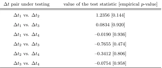
∆tpair under testing value of the test statistic [empiricalp-value] ∆t1vs. ∆t2 1.2356 [0.144]

∆t1vs. ∆t3 0.0834 [0.920]

∆t1vs. ∆t4 –0.0190 [0.936]

∆t2vs. ∆t3 –0.7655 [0.474]

∆t2vs. ∆t4 –0.3412 [0.806]

∆t3vs. ∆t4 –0.0754 [0.958]

there is no significant evidence to indicate that model (1) is misspecified for the TIF data set, as the null