Munich Personal RePEc Archive
Measuring the dependence structure
between yield and weather variables
Bokusheva, Raushan
ETH Zürich, Institute for Environmental Decisions
April 2010
Online at
https://mpra.ub.uni-muenchen.de/22786/
Measuring the dependence structure between yield and weather variables
Abstract
The design and pricing of weather-based crop insurance and weather derivatives is strongly based on an implicit assumption that the dependence structure between yields and weather variables remains unchanged over time. In this paper, we prove this assumption based on empirical time series of weather variables and farm wheat yields from Kazakhstan over the period from 1961 to 2003. By employing two different methods to measure dependence in multivariate distributions – the regression analysis and copula approach – we reveal statistically significant temporal changes in the joint distribution of relevant variables. These empirical results indicate that greater effort is required to capture potential temporal changes in the dependence between yield and weather variables, and subsequently to consider them in the design and rating of weather-based insurance instruments.
Key words: weather-based index insurance, dependence structure, copula estimation, Bayesian
hierarchical model, Kazakhstan.
1. Introduction
2 There are several options for reducing farm households’ exposure to weather risk. Among formal insurance schemes, so-called index-based crop insurance products have been considered as especially promising (Varangis et al., 2002), primarily because they are less vulnerable to moral hazard and adverse selection than common farm yield insurance (e.g. Skees et al., 1997, Skees et al., 1999). Recently, particular attention has been paid to crop insurance instruments based on weather indexes. Such instruments have been introduced as pilot programs in several countries. According to the United Nations (UN) Department of Economic and Social Affairs (2007), pilot projects on weather-based insurance have been implemented in India, Ukraine, Ethiopia, and Malawi. New pilot projects are planned for Nicaragua, Tanzania, Thailand, Bangladesh and Senegal (Barnett and Mahul, 2008).
The literature into the feasibility of weather-based insurance shows that, generally, this type of insurance might be very effective in reducing the farmers’ yield risk (Skees et al., 2001, Breustedt et al., 2008; Musshoff et al., 2009). Yet, some recent investigations employing cross- validation techniques to evaluate predictive power of the potential risk reduction estimates show that the estimates of the hedging effectiveness of weather derivatives and weather-based index insurance can considerably differ between the training and test data sets (Vedenov and Barnett, 2004; Bokusheva and Breustedt, 2008).
3 that inconsistency between in- and out-of-sample performance “…creates a potential problem in designing and marketing the contracts” (Vedenov and Barnett, 2004, p. 401).
Recently, Bokusheva and Breustedt (2008) have proposed evaluating the predictive power of the ex post risk reduction due to index-based insurance by comparing it with a so-called benchmark risk reduction. To this end, these authors distinguish between two consecutive periods in the time series and thus form a training data set and a test data set. Bokusheva and Breustedt estimate the ex post risk reduction based on the training data set and compare it with the benchmark risk reduction computed by employing the test data set. To measure the benchmark risk reduction, the study allows for annual updates of insurance contract parameters and the optimal number of insurance contracts to purchase. Empirical results by Bokusheva and Breustedt (2008) show that the ex post approach can seriously overestimate potential risk reduction due to index-based insurance schemes. In their study, the difference in risk reduction between ex post and benchmark estimates was especially pronounced for weather-based insurance instruments.
4 In fact, when pricing and evaluating index-based insurance, the literature implicitly assumes that the historically-determined pattern of farm yield dependence on a weather variable will remain unchanged over a certain time horizon. In our opinion, this assumption might be too restrictive. Yet, by now no attempt has been done to validate this assumption. We suppose that in the case of temporal changes in the joint distribution of yield and weather variables, the effectiveness of weather-based insurance might be affected critically, if such changes are not taken into account when designing and rating weather-based insurance contracts. Hence, in this study we suggest to prove this assumption by applying two alternative methods to measure stochastic dependence – the standard regression analysis and the copula approach. By employing the 43-year time series of weather and yield data for 10 grain producers in Kazakhstan, we show that this assumption does not hold for our empirical data.
The remainder of the paper is structured as follows: Section 2 provides an overview of the
methodology to measure the dependence structure in multivariate distributions. Section 3 details
the data and empirical procedure employed. In section 4, we present the results of our empirical
application. The final section concludes.
2. Methodology
2.1 Measuring the dependence structure
The crop insurance contract design strongly relies on a statistical analysis of the time series data. When designing index-based insurance, the standard regression analysis is applied to measure the sensitivity of farm yields to a particular index. Considering area yield insurance, the literature refers to the so-called critical β (Miranda, 1991), which represents the sensitivity of the farm
5 from one or several weather indicators. Skees et al. (2001) and Turvey (2001) use either cumulative rainfall or temperature, while Vedenov and Barnett (2004), Bokusheva (2006) and Xu et al. (2008) analyze the effectiveness of weather derivatives and insurance products based on a combination of several weather indicators. A weather index is constructed by applying a regression model, which allows to evaluate the sensitivity of the farm (county) yields to selected weather indicators. Thereby, empirical analyses implicitly assume that the dependence structure between considered variables can be captured well by linear correlation.
However, though very popular in applied economic research, linear correlation is only one particular measure of stochastic dependency. For long time, empirical investigations have neglected the fact that linear correlation is hardly applicable beyond the scope of multivariate normal distributions. However, empirical evidence shows that the distributions of the real world are seldom of this class (Embrechts et al. 2002). Hence, the use of linear correlation as a measure of dependence may cause a serious overestimation or underestimation of the dependency between the random variables of interest and thus lead to incorrect empirical results. Moreover, linear correlation is not adequate for representing dependency in the tails of multivariate distributions (McNeil et al, 2005), a quality that makes linear correlation hardly applicable in actuarial models that assess extremal insurance losses.
In recent years, the copula approach has become increasingly popular in modeling multivariate dependence structures, particularly in fields such as finance, biostatistics and actuarial mathematics (Trivedi and Zimmer, 2007). According to McNeil et al. (2005) a d-dimensional
copula C(u)C(u1,,ud) is a multivariate distribution function on d
1]
[0, with standard
6 The usefulness of copulas for modeling multivariate dependence stems from Sklar’s theorem (1959), which states that if F is a joint distribution function with marginal distributions F1,, Fd,
then there exists a copula C: [0,1]d [0,1]
such that for all x1,,xd in R
,
,
x1, ,xd
C
F1
x1 , ,Fd
xd
F . (1)
Accordingly, any continuous multivariate distribution can be uniquely described by two parts: the marginal distributions Fi and the multivariate dependence structure captured by the copula C.
Though empirical researchers often know the marginal distributions of individual variables, the joint behavior of relevant variables remains hidden. Copulas can be very helpful in this context, because they allow researchers to describe joint distributions when only marginal distributions are known. A crucial advantage of copulas is that the marginal distributions may come from various distribution families.
In general, it is distinguished between parametric and nonparametric (e.g. kernel) copulas. Empirical analyses however employ primarily parametric copulas. In turn, parametric copulas are divided into implicit and explicit types of copulas. Implicit copulas are copulas implied by the well-known multivariate distribution functions and do not themselves have simple closed forms (McNeil et al, 2005). The most widely applied implicit copulas are the Gaussian copula and Student’s t copula (hereafter referred to as t copula).
The Gaussian copula is given by:
d d
P
d
Ga
P P X u X u u u
C 1 1
1 1
1 ,..., ,...,
Φ
u , (2)
7 In principle, an implicit copula can be extracted in the same way from any other distribution with continuous marginal distribution functions. For example, the d-dimensional t copula takes the form:
vP
d
tP t u t u
C, u t , 1 1 ,...,1
, (3)
where tν is the distribution function of a standard univariate t distribution, tν,P is the joint distribution function of the vector X ~ td(ν, 0, P), and P is a linear correlation matrix.
In general, the t copula allows a more flexible representation of dependence than the Gaussian copula, because it does not assume that uncorrelated multivariate random variables are independent (McNeil et al., 2005). The t copula displays asymptotic upper tail dependence even for negative and zero correlations. In contrast, the Gaussian copula has the property of asymptotic independence. Embrechts et al. (2002) notice that regardless of how high a correlation is chosen, extreme events appear to occur independently in single marginal distributions for Gaussian copulas.
In contrast to the implicit copulas, the explicit copulas do have a simple closed form. An example of an explicit copula is the Clayton copula:
/ 1 1
1,... , ... 1
u u d
u u
C d d
Cl
with 0 , (4)
where θ denotes the dependence parameter to be estimated. As θ→ 0 it represents independence,
while as θ → ∞ it describes perfect dependence. The Clayton copula exhibits strong left tail dependence and relatively weak right tail dependence. Because of this property, it has been quite often used in financial applications (McNeil et al., 2005). It does not, however, allow negative dependence (McNeil et al., 2005).
8
/ 1 1
1,... d, exp ln ... ln d
Gu
u u
u u
C with 1 . (5)
Similar to the Clayton copula, the Gumbel copula cannot account for negative dependence. However, in contrast to the Clayton copula, the Gumbel copula exhibits strong right tail dependence and relatively weak left tail dependence.
Recently, Xu et al. (2009) used the copula approach to determine the magnitude of spatial dependence in the joint distribution of weather indices across different regions in Germany. While employing two explicit copulas, the Clayton and Gumbel copulas, the authors found that a Clayton copula is more appropriate for representing spatial dependence considering all three weather indices in their study. Consequently, the study applies this copula to estimate potential net aggregated losses of insurance companies when providing weather-based insurance. However, Xu et al. (2009) do not model the dependence structure between yields and weather variables. Instead, they assume that indemnity payments depend on the considered weather indices. Taking into account a relatively low dependency between weather indices and farm yields in Germany (Xu et al., 2008), this assumption seems to be too strong and might have introduced a bias into the authors’ estimates of aggregated losses.
9 because they do not require any assumptions and are primarily data driven. Yet, Trivedi and Zimmer (2007) emphasize that nonparametric copulas present a straightforward approach if the considered random variables are independent and identically distributed. However, ‘…this may be a reasonable assumption with cross section data, but may be more tenuous in time series applications’ (Trivedi and Zimmer, 2007, p. 60). Moreover, Trivedi and Zimmer (2007) point out problems related to the estimation of likelihoods for nonparametric copulas, which complicates their evaluation. In fact, Vedenov (2008) failed to obtain valid log-likelihood values when approximating yield distributions by means of the Normal, Gamma and Weibull distributions.
Zhu et al. (2008) applied Gaussian copula and t copula to define the dependence structure in multivariate distributions of crop yields and prices. By applying Akaike Information Criterion (AIC) and the log-likelihood test, these authors have found a better goodness-of-fit for a t copula than a Gaussian copula. This suggests a higher magnitude of dependency in the distribution tails. Consequently, by using both copulas to rate a revenue insurance contract, the authors demonstrate that the actuarially fair premium rates are lower for t copula than for the Gaussian copula.
10 since the impact of climate change is expected to be especially pronounced due to an increase in the quantity and severity of extremal events (IPCC, 2007), the dependence structure between yields and single weather variables may differ noticeably in the left tail of the distribution than in the middle or the right tail of their joint distribution. Accordingly, more effort will be required to model the tails’ dependence structure in future empirical research.
2.2 Bayesian modeling
Due to the seasonality of agricultural production, only relatively short time series are typically available for empirical studies. This often hampers the application of some advantageous methods applied in, e.g. financial research in the context of agricultural decision-making. In particular, the estimation of copula function parameters requires sufficiently long time series to assure a reasonable number of observations in the tails of joint distributions.
Applying the standard regression analysis in the context of the weather-based index insurance design and rating is also often subject to some serious limitations. As Vedenov and Barnett emphasize regarding the design of weather derivatives for U.S. agriculture, ‘…rather complicated combinations of weather variables must be used in order to achieve reasonable fits of the relationship between weather and yield.…’ (Vedenov and Barnett, 2004, p.399). However, a limited number of weather and yield observations - typically from 10 to 15 - does not provide a sufficiently high number of degrees of freedom, which might seriously affect the predictive power of the regression estimates.
11 units in an empirical sample population. An essential advantage of such estimations is that they allow researchers to ‘pool’ information across individual study units. At the same time, it is different from the standard polled estimations, which fully disregard potential differences across individual units.1
The Bayesian approach requires a sampling model for the observed data Y
y1,...,yn
and aprior distribution
on all unknown parameters θ in the model. The sampling model is givenin the form of probability distribution f(Y|θ). When regarded as a function of the vector of
parameters θ, this distribution is called likelihood. Compared to standard statistical analyses, the Bayesian approach does not consider θ as fixed parameters (i.e. scalars), but rather regards them
as random variables. This is done by adopting a prior distribution for every parameter in the vector θ. The prior distribution is a probability distribution that summarizes all information we have about a particular model parameter not related to that provided by the data Y. The prior distributions are used to compute the conditional distribution of the unknown parameters given the observed data, i.e. the posterior distribution p(θ|Y), from which all statistical inferences arise (Carlin and Louis, 2009):
d Y f Y f d Y p Y p Y p Y p Y p , , , . (6)According to equation (6), the posterior is a product of the likelihood f(Y|θ) and the prior
distribution
renormalized so that it integrates to one. Thus, both the observed data in theform of the likelihood, as well as prior information in the form of the prior distribution contribute to obtain inference about posterior distribution. In the basic Bayesian model, the prior distributions of the model parameters are specified by means of a vector of hyperparameters η
12 i.e.
η . Thus, the model has two stages, i.e. the parameters and hyperparameters. In thehierarchical Bayesian model, more than two stages are specified; therefore the hyperparameters in turn can depend on a vector of further unknown parameters specified by a second-step prior distributions, i.e. so-called hyperpriors. By supposing that parameters and hyperparameters for certain groups of study units have common prior and hyperprior distributions, respectively, the hierarchical Bayesian model ‘gains strength’ from the likelihood contributions of the respective units through their joint influence on the estimate of the unknown parameters and hyperparameters.
The Deviance Information Criterion (Spiegelhalter et al., 2002) is employed for the Bayesian model comparison. The DIC presents a generalization of Akaike Information Criterion based on
the posterior distribution of the deviance statisticsD
2logf(Y)2logh(Y), where f(Y|θ)is the likelihood function for the observed data vector Y given the parameter vector θ and h(Y) is a function used for standardizing the data. The DIC approach captures the fit of the model by the
posterior expectation of the deviance statistic, DEY
D , and by the effective number ofparameters defined as pD DD
, where D
D(EY
). Though the DIC does not13 3. Data and empirical procedure
3.1 Data
For our empirical application we used wheat yield data for 12 large grain producers in Central Kazakhstan. The yield data were collected from rayon2 statistical offices and covers the period from 1961 to 2003.3 As our data covers quite a long period, including the period of economic transformation in Kazakhstan, we tested the yield time series for structural breaks and removed two farms for which we revealed a statistically significant structural break. Thus, the data for only 10 farms were available for our empirical application. To account for the time component in the farms’ yield time series, we conducted a detrending procedure considering the second- and third-degree polynomial functions. Additionally, the cumulative rainfall variables for single months during the vegetation period (April to September) were used to improve the accuracy of trend parameters’ estimates. The second-degree polynomial trend provided a better statistical fit and thus was chosen to adjust the farms’ yields to their 2003 level.
As in 2003, the considered farms had 25,250 hectares of wheat crop area. The average farm wheat yield varied from 0.67 t/ha to 1.07 t/ha across the farms in the study period.
In addition to the farm yield data, the weather data from the corresponding weather station was used in the analysis. The weather data (daily rainfall and average daily temperature as reported to the regional meteorological offices) covered the same period as the yield data. The cumulative precipitation during the summer months (June to August) averaged 120 mm and varied between 48 mm and 239 mm from 1961 to 2003.
2Rayons are administrative districts similar to counties.
3 We have access to the data for a substantially larger group of farms in Kazakhstan, yet for most of them available
14 We used the available weather data to construct three different weather variables: cumulative rainfall index, rainfall deficit index and a drought index. We calculated all three selected indices considering different periods during the wheat vegetation season, i.e. from April to September.4 A detailed description of these indices appears in Appendix A1.
3.2 Empirical procedure
To measure the dependence structure between weather and yield variables, we first employ the copula approach. We use the Clayton and Gumbel copula to estimate tail dependence in the joint distributions of our empirical farm yield time series and selected weather variables. By doing so, we determine those weather indices which influenced yield losses of the study farms most strongly during the period under investigation. Subsequently, we estimate the coefficients of tail dependence between the farms’ yields and selected weather variables considering two consecutive sub-periods in our time series: from 1961 to 1982, and from 1983 to 2003. Then, we apply the standard two-sample t-test to check whether changes in the estimates of the tail dependence between these two sub-periods are statistically significant.
Subsequently, we apply the standard regression analysis to test for potential temporal changes in the sensitivity of the farms’ yields to a selected weather variable. Therefore, we employ two alternative model formulations. In the first model, we do not account for the effect of time when measuring the sensitivity of the farms’ yield to the selected weather indicator, i.e. we assume that it was constant over the considered period:
t
t w
y 01 , (6)
4 Time series of the farm yields and the selected weather indices were tested for non-stationarity by employing the
15 where ytis the vector of the farm yields, wtis the vector of respective weather observations, 0
and 1 are the intercept and the regression coefficients, respectively, and the subscript t indicates
time.
In the alternative model specification of the regression equation, we assume that the regression
coefficient 1 measuring the sensitivity of farm yields to a weather variable is not a constant, but
a function of time. Assuming that 1 is a function of time, i.e. 1 f(t,), we obtain:
t t f t w
y 0 (,) . (7)
We test various functional forms such as linear, logarithmic and quadratic to capture the effect of time on the sensitivity of yields to weather. Then, the estimation results of the dynamic model specification in (7) are tested against those of the static model formulation in (6).
In our study, we have a relatively long time series of the yield and weather variables that had to reduce problems related to low degrees of freedom and a low number of extreme observations in the regression and copula estimations, respectively. Yet, to increase the efficiency and consistency of our estimations, we suggest to estimate both copula and regression parameters by applying the Bayesian hierarchical models.
3.2.1 Bayesian copula estimation
To specify the Bayesian model for the copula estimation, we consider a bivariate vector (Y, W) representing a yield and a weather variable, respectively. Then, the joint probability function
Y Wθ
f , for these two variables can be defined as:
Y Wθ
c
F
Yθ F Wθ θ
f Yθ f Wθf , Y , W Y W
16 where θ is the vector of copula and marginal distributions’ parameters, and f and F denote a particular probability and cumulative marginal distribution function, respectively; and c is a copula density. Then, regarding a sample of size N and length T, the respective likelihood function is given by:
NxT
it W it X it
W it
X x F w f x f w
F c W
X
L , θ 1 θ, θ θ θ θ
. (8)
This is used to obtain the posterior distribution, defined as:
θX W
L X Wθ
g
θg , ,
, (9)
where g
θ is the prior distribution.The copulas are usually estimated by a two-step procedure: in the first step, the parameters of marginal distributions are obtained by fitting a parametric distribution to the empirical data; in the second step, the parameters of the copula function are estimated by means of the Maximum Likelihood (ML) method. In this research, we also apply the two-step procedure. Yet, instead of the ML method, Markov chain Monte Carlo (MCMC) algorithms were employed to obtain the joint posterior distributions of copula parameters (Gamerman and Lopez, 2006).5
The fitting and ranking (by goodness-of-fit test) of different probability distributions to our time series in @risk showed that the Weibull and LogLogistic distributions are mostly suitable for representing empirical distributions of the farms’ yields.6 The LogLogistic distribution provided a good fit for two weather indices: the cumulative rainfall and drought index, whereas the
5 The model estimations were done in WinBUGs (Spiegelhalter et al., 2003).
6
The yield marginal distribution parameters differ across the study farms. However, their estimation was done
17 Weibull distribution was identified to describe at best the rainfall deficit index. Accordingly, these two distribution families were employed in the first-step estimations.
In the second step, we then estimated copula parameters. To derive the likelihood function, the copula density is determined as the derivative of C with respect to each of its arguments, viz.:
v u v u C v u c , , 2, (10)
where C
u,v is a bivariate copula function, u and v are uniform marginal distributions of farms’yield and weather indices, respectively, i.e. uFY
ytY
and vFW
wtW
, where Yand Ware the vectors of the parameter estimates for marginal distributions of the farms’ yields and selected weather indices, respectively.
Accordingly, for the Clayton copula we obtained the following density function:
21 1 11 1
,v u v u v
u
cCl ,
with denoting the dependence parameter of the Clayton copula.
The Gumbel copula density is defined as follows:
1 1 1 2 ln ln ln ln ln ln exp 1 ln ln 2 , 1 1 v u v u v u v u v u v u cGu , (11)with representing the dependence parameter of the Gumbel copula, and u and v denoting
marginal survival functions (McNeil et al., 2005, p. 62) of farms’ yields and selected weather
variables, respectively, i.e. u FY
yt 1FY
ytY
and vFW
yt 1FW
wtW
. We18 measurement of the dependence structure in the upper tail of joint distributions. Thus, when replacing the distributions of farms’ yields by their survival distributions, we represent the downwards yield risk by the upper tail of the yields’ marginal distributions. The same is valid for two of the selected weather indices - the cumulative rainfall index and the drought index. Considering the rainfall deficit index, the marginal survival distribution of this index was employed in (10), while its marginal distribution was used in (11).7
The gamma distribution was used as the prior distribution of the dependence parameter for the
Clayton copula, i.e. ~Gamma(r,). The respective hyperpriors are r~Gamma(2, 2) and
) 100 , 2 (
~Gamma
. By choosing a quite large value of the scale hyperparameter, we obtain a
rather flat probability density of the gamma distributions, which in turn enables us to form rather non-informative priors.8
We employed the uniform distribution as the prior in the Gumbel copula model, which allowed us to easily account for the left-hand censoring of the dependence parameter in the Gumbel copula. In this case, the prior is ~U(a,b)and the hyperpriors are a~U(1, 10) and
) 100 , 10 ( ~U
b .
The Clayton copula parameter estimates were used to calculate the coefficients of lower tail
dependencel
0,1 measured in the left tail of the joint distribution of yield and weathervariables as:
7 For two of the selected weather indices – the cumulative rainfall index and drought index – lower values
correspond in general with lower values of yields. So in this case we employ the marginal survival distributions of both farms’ yields and weather indices in the Gumbel copula model. Yet, in the case of the rainfall deficit index, higher values of the index correspond with lower values of yields generally (i.e. the higher the rainfall deficit, the lower the yields). Hence, regarding this weather index, we employ the marginal distribution of the index and the survival marginal distributions of the yields to estimate the Gumbel copula, whereas we use the marginal survival distribution of the index and the marginal distributions of the yields to estimate the Clayton copula.
8 The use of rather non-informative priors and hyperpriors is essential if one wants to exercise minimum influence on
19
qq q C q F W P q F W q F Y P W Y q W W Y q l ) , ( lim ) ( ) ) ( ) ( ( lim ) , ( 0
0
, (12)
where q is the chosen quantile level (McNeil et al., 2005). According to (10), the coefficient of the lower tail dependence is defined as probability of the variable Y exceeding its q-quantile, given that the weather variable W exceeds its q-quantile when moving to the left tail of the joint distribution.
The upper tail dependence coefficient u
0,1 is defined as the probability that the variable Yexceeds its q-quantile given that the variable W exceeds its q-quantile when moving to the right tail of the joint distribution:
qq q C q q F W P q F W q F Y P W Y q W W Y q u 1 ) , ( 2 1 lim ) ( ) ) ( ) ( ( lim ) , ( 1 1 . (13)
The stronger is the dependence in the left tail of the joint distribution of the farm yields and a particular weather indicator, the closer the value of the respective tail dependence coefficient will be to one. Hence, a comparative analysis of the values of the coefficient can provide a valuable basis for selecting weather indicators, which are relevant for insurance contract design.
3.2.2 Bayesian regression
20 To capture the effect of time, three alternative functional forms, linear, logarithmic, and quadratic, are employed:
t
tt t w
y 0 0 , (13)
t
tt t w
y 0 0 ln , (14)
t tt
tt t t w
y 0 0 2 , (15)
respectively.
We also test whether the time effect has a systemic character, i.e. whether coefficients t andtt
are of the same magnitude or exhibit significant differences across the study farms, respectively. The comparison of the model specifications is done based on the DIC, but also by minimizing the posterior predictive loss measured as the mean squared predictive error (MSPE). Therefore, we computed the MSPE as the expected sum of squared deviations of the predicted yields from the observed yields for each year from 1996 to 2003.
4. Estimation results
21 dependence coefficient9 are found for the cumulative rainfall index calculated for the summer months from April to July, the Selyaninov drought index measured for June and July, and the rainfall deficit index computed from May to July, respectively. The individual posterior means of the tail dependence coefficient are highly significant with Monte Carlo (MC) errors lower than 0.001; their convergence was obtained for 5,000 MC iterations. Therefore, in the following we refer to the weather indices, which were calculated for the period noted above, respectively.
Table 1 about here
Table 1 summarizes the estimates of the Clayton and Gumbel copula for individual farms. According to both copula estimates, the cumulative rainfall index (calculated from April to July) provides the highest level of tail dependence. The average posterior mean estimates of the coefficients of the lower and upper tail dependence amount to 0.66 and 0.70, respectively, across farms. This indicates that – if this index falls below its expected value – the study farms’ yields fall below their respective expected values with a probability of approximately 0.70. The estimates for the Selyaninov drought index and the rainfall deficit index are rather similar and amount to ca. 0.62 and 0.69 for the Clayton and Gumbel copulas, respectively, in each case. An interesting result is that the estimates of tail dependency do not vary much across farms, which is often the case if the weather indices are fitted to individual farm yields by linear regression. Although for all considered weather indices, the Gumbel copula estimates are associated with lower values of the DIC compared to the Clayton copula estimation results, a direct comparison
9 The posterior mean estimates of the tail dependence were quite robust to the changes of the quintiles at which the
22 of the estimation results from both models in terms of the DIC is not possible, as the DIC is not neutral to the reparameterization.10
Table 2 and 3 about here
Tables 2 and 3 present the estimation results of the Clayton and Gumbel copula models involving two parameters of dependence: one from 1961 to 1982, and the other from 1983 to 2003, respectively. The estimations of the tail dependence coefficient differ significantly across these two periods across almost all copula model estimates according the two-sample-mean difference t-test. Considering the Clayton copula (Table 2), the hypothesis H0 about equal sample means were rejected for all three weather indices at the 0.01-level of significance. The Gumbel copula model does not provide as distinctive results as does the Clayton copula model estimation (Table 3). The two-sample-mean test could not reject H0: for the cumulative rainfall index, however, it was rejected in the case of the Selyaninov drought and rainfall deficit indices, at the 0.05 and 0.01 confidence levels, respectively. Except the estimates for the cumulative rainfall index based on the Gumbel copula, the estimates indicate a significant increase in the tail dependence between the farms’ yields and the weather indices in the second sub-period. These results suggest that the dependence structure in the joint distributions of weather and yield variables was not constant from 1961 to 2003, and the dependence of the farm yields on weather was more pronounced in the second sub-period.
Moreover, our estimates show that changes in tail dependence are uneven regarding single weather indices. The shift in the tail dependence coefficient was especially pronounced considering the Clayton copula estimates. Figure 1 shows that the shift in the tail dependence coefficient was strongest for the rainfall deficit index and less evident for the cumulative rainfall
10 While the Clayton copula is defined based on absolute values of marginal distributions, the Gumbel copula
23 index (see also Figures A1 and A2 in the Appendix).11 This result implies that there can be differences in that how well single weather indices represent extreme dependence between yields and weather in different periods.
Figure 1 about here
Now we turn to the estimation results of the Bayesian regression models. To reduce the scope of the analysis, the regression estimations were done considering only the cumulative rainfall index that exhibited the strongest influence on the farms’ yields according to the copula estimations. First we estimated the specifications of the regression model (6) and (13) to (15) for the entire period from 1961 to 2003. The estimations were carried out considering that the effect of time can have either an idiosyncratic or a systemic effect. Accordingly, we estimated regression
models with individual coefficientst andtt for each study farm, but also with the same
coefficients t andtt over all study farms. According to the DIC, all three specifications, i.e.
from (13) to (15), provided a better fit than the specification in (6) considering both the idiosyncratic and systemic formulations of the time effect, respectively (Table 4).12 Moreover, thet andtt coefficient estimates are highly significant across all model specifications with
time effect. In addition, the dynamic specifications of the model allow the reduction of the MC-errors of the intercept estimates for individual farms: while the intercept estimates in the static
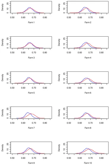
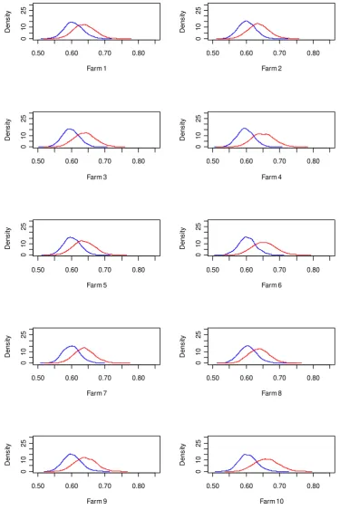
11 While Figures 1 presents the distribution of the posterior mean estimates of the tail dependence coefficient across
farms, Figures A1 and A2 (Appendix) show the posterior distributions of the tail dependence coefficient for each single farm. For both representations, we can observe a more pronounced shift in the distribution of the tail dependence coefficient for the rainfall deficit index compared to the cumulative rainfall index.
12 We present the estimates of the specification in (14), as it has been proven to be superior to the specifications in
24 specification are significant at the 0.10-level for most of study farms, in the dynamic formulation the corresponding estimates become significant at the 0.05-level.13
Table 4 about here
Among the three functional forms employed, the logarithmic was found to capture dynamics in the sensitivity of the farm yields to the weather index considered as best according to the DIC. In addition, we could not find serious differences in the systemic and idiosyncratic formulations of the model; indeed, for the logarithmic specification (14), the DIC values are found to be almost the same, i.e. 2,132.4 and 2,131.9, respectively (Table 4).
To assess the posterior predictive loss, we estimated model specifications (6) and (14), i.e. without time effect and with time effect, captured by means of the logarithmic function, for the sub-period from 1961 to 1995. We then used the yields’ predictions of respective models to compute the MSPE for the consecutive sub-period from 1996 to 2003. Table 5 summarizes the respective estimates. Tin general the estimation results for the sub-period from 1961 to 1995 are very similar to those for the whole period, i.e. from 1961 to 2003. In terms of the DIC, both dynamic formulations of the model – with idiosyncratic and a systemic effect of time – outperform the static formulation. Yet, the static formulation provides lower prediction errors: the MSPE criterion is lower for this formulation than in both dynamic formulations. These results suggest that, though there are temporal changes in the sensitivity of the farms’ yields to the selected weather index, predicting the future trajectory of such temporal changes can be complicated and might increase the predictions’ uncertainty.
13 All other parameters are found to be highly significant (i.e. at the 0.01-level) according to the MC-error statistic for
25 Conclusions
When pricing and evaluating index-based insurance, the literature implicitly assumes that the joint distribution of farm yields and a weather variable captured by means of empirical time series will remain unchanged in future. In this paper, we attempt to validate this assumption by employing the copula approach, as well as by a dynamic regression model formulation. The empirical exercise is completed based on the wheat yield and weather time series for 10 large grain-producing farms in Kazakhstan for the period from 1961 to 2003.
According to our estimates, the dependence structure in the joint distributions of the study farms’ yield and weather variables was changing during the considered period. The estimation results based on two copula models – the Clayton and Gumbel copulas – suggest that the dependence of the farm’s yields on weather was significantly higher from 1983 to 2003 compared to the period from 1961 to 1982 regarding almost all weather indices considered in this study. We also obtained significant positive estimates for the regression parameters representing the effect of time on the sensitivity of farm yields to weather. Consequently, the estimations’ results for both the copula and regression models imply an increase in the dependency of the study farms’ yields on the selected weather variables during the study period. We suppose that as such temporal changes might become even more pronounced and fast due to climate change, neglecting them – when rating weather-based insurance – might lead to an undervaluation of the involved risks, and thus might negatively affect the actuarial fairness of the insurance premium.
27 References
Barnett BJ, Mahul O. Weather Index Insurance for Agriculture and Rural Area in Lower-Income Countries. American Journal of Agricultural Economics, 2007; 89:1241-1247.
Bokusheva R, Breustedt G. Ex ante evaluation of index-based crop insurance effectiveness, contributed paper for the XII EAAE Congress ‘People, Food and Environments: Global Trends and European Strategies’, Ghent (Belgium), August 26-30, 2008.
Breustedt G, Bokusheva R, Heidelbach O. The potential of index insurance schemes to reduce farmers’ yield risk in an arid region. Journal of Agricultural Economics, 2008; 59:312-328. Carlin BP, Louis TA. Bayesian methods for data analysis, 3rd edition. CRC Press, Taylor & Francis Group: Boca Raton, 2009.
Embrechts P, McNeil AJ, Straumann D. Correlation and dependency in risk management: properties and pitfalls. Pages 176–223 in Dempster M (ed). Risk Management: Value at Risk and Beyond Cambridge University Press, 2002.
Gamerman D, Lopes HF. Markov Chain Monte Carlo: Stochastic Simulation for Bayesian Inference, 2nd eds. Chapman & Hall, London, 2006.
IPCC. Climate Change 2007 – Mitigation of Climate Change. Contribution of Working Group III to the Fourth Assessment Report of the IPCC. IPCC, Geneva, Switzerland, 2007.
McNeil A, Frey R, Embrechts P. (2005). Quantitative Risk Management, Princeton University Press, Princeton, 2005.
Miranda MJ. Area-Yield Crop Insurance Reconsidered. American Journal of Agricultural Economics, 1991; 73:233-242.
Musshoff O, Odening M, Xu W. Management of climate risks in agriculture – will weather derivatives permeate? Applied Economics, (2009); 1-11, iFirst. DOI: 10.1080/00036840802600210.
Shamen AM. Ob Issledovanii Zasushlivih Yavlenij v Kazakhstane (Research on Drought in Kazakhstan). Hydrometeorology and Ecology, 1997; 2:39-56.
Skees JR, Gober S, Varangis P, Lester R, Kalavakonda V. Developing Rainfall-Based Index Insurance in Morocco. Policy Research Working Paper 2577. World Bank, 2001.
Skees JR, Black JR, Barnett BJ. Designing and Rating an Area Yield Crop Insurance Contract. American Journal of Agricultural Economics, 1997; 79:430-438.
Skees, JR, Hazell P, Miranda M. New Approaches to Crop Yield Insurance in Developing Countries. EPTD Discussion Paper No. 55, Environment and Production Technology Division, International Food Policy Research Institute, Washington, D.C.S, 1999.
Sklar A. Fonctions de répartition à n dimension et leurs marges, Publ. Inst. Stat. Univ. Paris, 1959; 8:299-231.
Spiegelhalter DJ, Best NG, Carlin BP, Linde A. Bayesian measures of model complexity and fit (with discussion). Journal of Royal Statistical Society, 2002; 64:583–639.
28 Turvey CG. Weather Derivatives for Specific Event Risks in Agriculture, Review of Agricultural Economics, 2001; 23:333–351.
Trivedi PK, Zimmer DM. Copula Modeling: An Introduction for Practitioners. now Publishers Inc., Delft, The Netherlands, 2007.
UN Department of Economic and Social Affairs. Developing Index-Based Insurance for Agriculture in Developing Countries. Sustainable Development Innovation Briefs, 2007; 2:1-8. Varangis P, Skees J, Barnett B. Weather Indexes for Developing Countries. In Dischel R (ed). Climate Risk and the Weather Market. London: Risk Books, 2002.
Vedenov DV. Application of copulas to estimation of joint crop yield distributions, Contributed paper at the Annual Meeting of the AAEA 2008, Orlando, USA, July 27-29, 2008.
Vedenov DV, Barnett BJ. Efficiency of weather derivatives as primary crop insurance instruments. Journal of Agricultural and Resource Economics, 2004, 29:387-403.
Xu W, Odening M, Musshoff O. Indifference pricing for weather derivatives. American Journal of Agricultural Economics, 2008; 90:979-993.
Xu W, Filler G, Odening M, Okhrin O. On the systemic nature of weather risk. Agricultural Finance Review, 2010; 70 (in print).
29 Table 1: Summary statistics of the tail dependence posterior mean estimates1) for selected
weather indices (10 farms, 1961-2003)
Mean SD Min Max DIC
Clayton copula
Cumulative Rainfall, April-July 0.662 0.007 0.649 0.675 830
Selyninov Index, June-July 0.629 0.008 0.616 0.639 920
Rainfall Deficit, May-July, k=0.92) 0.619 0.005 0.613 0.629 920
Gumbel copula
Cummulative Rainfall, April-July 0.697 0.005 0.692 0.707 390
Selyninov Index, June-July 0.685 0.003 0.680 0.688 410
Rainfall Deficit, May-July, k=0.92) 0.686 0.003 0.682 0.692 410
1)
The Monte Carlo error < 0.001 for single estimates
2)
k stands for strike level, s. Appendix A1 Source: own estimates
Table 2: The posterior mean estimates of the tail dependence coefficient for selected weather indices, two period estimates1), Clayton copula
Cumulative Rainfall2) Selyaninov Index2) Rainfall Deficit2)
1961-1982 1983-2003 1961-1982 1983-2003 1961-1982 1983-2003
Farm 1 0.659 0.669 0.621 0.641 0.607 0.638
Farm 2 0.649 0.663 0.608 0.638 0.602 0.636
Farm 3 0.661 0.665 0.618 0.641 0.598 0.640
Farm 4 0.655 0.673 0.617 0.645 0.598 0.650
Farm 5 0.653 0.662 0.609 0.637 0.602 0.637
Farm 6 0.662 0.676 0.614 0.646 0.603 0.653
Farm 7 0.649 0.676 0.614 0.646 0.600 0.639
Farm 8 0.659 0.670 0.614 0.641 0.605 0.638
Farm 9 0.653 0.669 0.618 0.637 0.602 0.642
Farm 10 0.669 0.690 0.623 0.654 0.605 0.661
Mean, µ 0.657 0.671 0.616 0.642 0.602 0.643
SD 0.006 0.008 0.005 0.005 0.003 0.009
H0: µ1961-1982 = µ
1983-2003 rejected
3)
rejected3) rejected3)
1)
The Monte Carlo error < 0.001 for single estimates
2)
The weather indices refer to the same periods as in Table 1, respectively.
3) at the 0.01-significance level
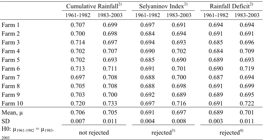
[image:30.595.69.510.389.628.2]30 Table 3: The posterior mean estimates of the tail dependence coefficient for selected weather indices, two period estimates1), Gumbel copula
Cumulative Rainfall2) Selyaninov Index2) Rainfall Deficit2)
1961-1982 1983-2003 1961-1982 1983-2003 1961-1982 1983-2003
Farm 1 0.707 0.699 0.697 0.691 0.694 0.694
Farm 2 0.700 0.698 0.684 0.694 0.691 0.691
Farm 3 0.714 0.697 0.694 0.693 0.685 0.696
Farm 4 0.702 0.707 0.690 0.702 0.684 0.709
Farm 5 0.702 0.693 0.685 0.690 0.689 0.693
Farm 6 0.713 0.711 0.691 0.701 0.690 0.719
Farm 7 0.697 0.708 0.688 0.700 0.687 0.694
Farm 8 0.705 0.708 0.688 0.698 0.691 0.699
Farm 9 0.703 0.700 0.692 0.689 0.689 0.695
Farm 10 0.720 0.733 0.697 0.716 0.691 0.722
Mean, µ 0.706 0.705 0.691 0.697 0.689 0.701
SD 0.007 0.011 0.004 0.008 0.003 0.011
H0: µ1961-1982 = µ
1983-2003 not rejected rejected
3)
rejected4)
1)
The Monte Carlo error < 0.001 for single estimates
2)
The weather indices refer to the same periods as in Table 1, respectively.
3)
at the 0.05-significance level
4)
31 Table 4: Regression model estimates1): static and dynamic formulations, 1961-2003
static dynamic
systemic idiosyncratic
const[1] 3.396 * 3.348 ** 2.841 ** const[2] 3.059 ** 3.096 ** 2.481 ** const[3] 2.119 ** 2.152 ** 2.315 ** const[4] 1.439 ** 1.345 ** 1.736 ** const[5] 2.230 ** 2.309 ** 2.330 ** const[6] 1.568 ** 1.510 ** 1.883 ** const[7] 1.810 ** 1.765 ** 2.004 ** const[8] 3.380 * 3.268 ** 2.840 ** const[9] 1.634 ** 1.700 ** 2.052 ** const[10] 1.223 *** 1.151 *** 1.597 ** alpha[1] 0.051 *** 0.037 *** 0.036 *** alpha[2] 0.051 *** 0.037 *** 0.035 *** alpha[3] 0.044 *** 0.032 *** 0.034 *** alpha[4] 0.040 *** 0.027 *** 0.031 *** alpha[5] 0.044 *** 0.032 *** 0.033 *** alpha[6] 0.041 *** 0.028 *** 0.032 *** alpha[7] 0.040 *** 0.027 *** 0.031 *** alpha[8] 0.051 *** 0.036 *** 0.036 *** alpha[9] 0.040 *** 0.028 *** 0.032 *** alpha[10] 0.040 *** 0.027 *** 0.031 ***
beta_systemic ‐‐ 0.005 *** ‐‐
beta[1] ‐‐ ‐‐ 0.007 ***
beta[2] ‐‐ ‐‐ 0.007 ***
beta[3] ‐‐ ‐‐ 0.003 ***
beta[4] ‐‐ ‐‐ 0.003 ***
beta[5] ‐‐ ‐‐ 0.003 ***
beta[6] ‐‐ ‐‐ 0.002 ***
beta[7] ‐‐ ‐‐ 0.003 ***
beta[8] ‐‐ ‐‐ 0.007 ***
beta[9] ‐‐ ‐‐ 0.002 ***
beta[10] ‐‐ ‐‐ 0.002 ***
DIC 2149 2132 2132
MSPE (1996‐2003) 461 537 522
1)
the number in the brackets corresponds with the respective farm number; *, **, *** - significant at the 0.01, 0.05 and 0.10-significance level according to the Monte Carlo error, respectively;
2)
dynamic model formulation presented in the table refers to the logarithmic specification of the effect of time;
3)
32 Source: own estimates
Figure1: Posterior mean estimates of the tail dependence coefficient between farm yields and three considered weather indices: Cumulative Rainfall Index (CRI), Selyaninov Drought Index (Sel) and Rainfall Deficit Index (RDI); two period estimates, Clayton copula
.6
.6
2
.6
4
.6
6
.6
8
.7
CRI 1961-1982 CRI 1983-2003
Sel 1961-1982 Sel 1983-2003
RDI 1961-1982 RDI 1983-2003
33 Appendix
Appendix A1: Specification of weather indices
The cumulative rainfall index (CRI) was calculated as the sum of the monthly cumulated rainfall (MCR), viz.:
j
jt t MCR
CRI
where t and j are the year and the month subscripts, respectively.
The Selyaninov drought index (SDI) was computed according to Selyaninov (1958) (quoted in Shamen, 1997) as the ratio of cumulative rainfall in a particular period and the sum of the average daily temperatures in each month in the same period:
j
jt j
jt t
Temp MCR SDI
* 10
,
where Tempjt is the sum of the daily average temperatures in month j.
The rainfall deficit index (RDI) is a cumulated sum of the monthly rainfall deficit (MRD) determined as follows:
) 0 ; max( j jt
jt kw w
MRD ,
where wj is the long-term mean cumulated rainfall for month j, wjtis the actual realization of the
cumulated rainfall in the respective month, and k is the factor which was set to three alternative strike levels: 0.9, 1.0, and 1.1. Then, the rainfall deficit index (RDI) is obtained as:
j
jt t MRD
34 Figure A2-1: Posterior distributions of the tail dependence coefficient between farm yields and the Cumulative Rainfall Index; two period estimates (1961-1982: blue line; 1983-2003: red line), Clayton copula.
0.50 0.60 0.70 0.80
01 0 2 5 Farm 1 D ens ity
0.50 0.60 0.70 0.80
01 0 2 5 Farm 2 D ens ity
0.50 0.60 0.70 0.80
01 0 2 5 Farm 3 D ens ity
0.50 0.60 0.70 0.80
01 0 2 5 Farm 4 D ens ity
0.50 0.60 0.70 0.80
01 0 2 5 Farm 5 D ens ity
0.50 0.60 0.70 0.80
01 0 2 5 Farm 6 D ens ity
0.50 0.60 0.70 0.80
01 0 2 5 Farm 7 De n s ity
0.50 0.60 0.70 0.80
01 0 2 5 Farm 8 De n s ity
0.50 0.60 0.70 0.80
01 0 2 5 Farm 9 D ens ity
0.50 0.60 0.70 0.80
35 Figure A2-2: Posterior distributions of the tail dependence coefficient between farm yields and the Rainfall Deficit Index; two period estimates (1961-1982: blue line; 1983-2003: red line), Clayton copula.
0.50 0.60 0.70 0.80
01 0 2 5 Farm 1 D ens ity
0.50 0.60 0.70 0.80
01 0 2 5 Farm 2 D ens ity
0.50 0.60 0.70 0.80
01 0 2 5 Farm 3 De n s ity
0.50 0.60 0.70 0.80
01 0 2 5 Farm 4 De n s ity
0.50 0.60 0.70 0.80
01 0 2 5 Farm 5 D ens ity
0.50 0.60 0.70 0.80
01 0 2 5 Farm 6 D ens ity
0.50 0.60 0.70 0.80
01 0 2 5 Farm 7 De n s ity
0.50 0.60 0.70 0.80
01 0 2 5 Farm 8 De n s ity
0.50 0.60 0.70 0.80
01 0 2 5 Farm 9 De n s ity
0.50 0.60 0.70 0.80