Scalable Algorithms for Missing Value Imputation
ABSTRACT
Statistical Imputation Techniques have been proposed mainly with the aim of predicting the missing values in the incomplete sets as an essential step in any data analysis framework. K-means-based Imputation, as a representative statistical imputation method, has been producing satisfied results in terms of effectiveness and efficiency in handling popular and freely available data set (e.g., Bupa, Breast Cancer, Pima, etc.). The main idea of K-means based methods is to impute the missing value relying on the prototypes of the representative class and the similarity of the data. However, such kinds of methods share the same limitations of the K-means as data mining technique. In this paper and motivated by such drawbacks, we introduce simple and efficient imputation methods based on K-means to deal with the missing data from various classes of data sets. Our proposed methods give higher accuracy than the one given by the standard K-means.
General Terms
Data Mining, Algorithms
Keywords
Statistical Imputation, Clustering, K-mean
1.
INTRODUCTION
The quality of mining a data set in any data analysis framework is affected by how complete the data is. As a consequence, the quality of the data attracts the attention of many scientists working on Data mining and other correlated area such as Machine learning. The presence of missing data presents a challenge in the cleaning step, which is occurred in the phase of data collection [1, 2]. As pointed out in [3, 4, 5], we can classify the missing data into three categories: Missing completely at random (MCAR), Missing at random (MAR), and Not missing at random (NMAR).
In the MCAR, the absence of an item is not associated with any other item in the data set, observed or missing. In other words, the distribution of an example when containing a missing value for an attribute does not depend on either the observed data or the missing data. On the other hand, MAR has a less restrictive assumption than MCAR. It indicates that the absence of an item depends only on the observed values in the data set (e.g., the dependency is only for the observed data). Compare to MAR, NMAR produces the opposite condition, which the absence of an item reflects its probable data value [4].
In order to deal with such issues, several treatment missing data methods have been proposed, they can be divided into three categories: First, Ignoring and discarding (ID) category. There are two main ways to discard data with missing values. The first is discarding all instances with missing data while the second is discarding instances and/or attributes. This method relies on the definition and the specification of the high levels of missing data to evaluate its relevance to the
analysis. However, the most relevant attributes should be kept even with high degree of missing values. The second category is Parameter Estimation (PE) class. In this class, Maximum likelihood procedures are used to estimate the parameters of a model defined for the complete data (e.g., Expectation-Maximization [6] algorithm is applied in [2] to handle parameter estimation in the presence of missing data). The last category is Imputation [7, 8, 9], which is proposed with the aim of filling the missing values with estimated ones. The methods presented in this paper focus mainly on the last category.
2.
STATISTICAL IMPUTATION
METHODS
Statistical Imputation is the process of replacing missing values with estimated ones based on some statistical information available in the data set. There are many options varying from naive methods like mean or mode imputation [10] to some more robust methods based on relationships among attributes. Also, Imputation type is determined by how many values to be predicted for the missing one (e.g., single/multiple imputation [11]). In this section, we briefly describe different kind of imputation methods and highlight their limitations.
Mean and mode imputation (Mimpute) [12, 13, 14] consists of replacing the unknown/missing value for a given attribute by the mean (quantitative attribute) or mode (qualitative attribute) of all known/available values of that attribute. However, replacing all missing records with a single value distorts the input data distribution. Hot deck imputation (HDimpute) [15] replaces the missing data with the values from the input vector that is closest in terms of the attributes that are known in both patterns. Unlike Mimpute, this method attempts to preserve the distribution by substituting different observed values for each missing item [12]. Another solution is provided by Cold Deck imputation (CDimpute) method, which is similar to hot deck but the data source must be other than the current data set. On the other hand, Prediction models [11, 14] consist of creating a predictive model in order to estimate values that will substitute the missing data. The main idea of the predictive model is to rely on the correlations presented among the attributes to create a predictive model for classification or regression. However, its main disadvantage is that a huge number of prediction models have to be designed when missing items appear in many combinations of attributes in a high dimensional problem.
Abdel-Rahiem A. Hashem
Mathematics Department, AssiutUniversity, Assiut, Egypt
Marghny H. Mohamed
Faculty of Computers and Information, Assiut University, Assiut, Egypt
Mohammed M. Abdelsamea
IMT Institute for Advanced Studies,2.1.
K-Means based Imputation
In this section, we review the main idea of the K-means based imputation methods. Once the clusters are constructed, the imputation can be done by the corresponding prototypes from the most similar k-centroid of the given classes. The Classic Imputation algorithm (CI) can be described as follows:
1. Divide dataset S into Complete-valued dataset St, and Missing-valued dataset S∗.
2. Apply classical k-mean on complete dataset St until convergence and obtain wj centers, j ∈ {1, 2, ..., k}.
3. For each instance xi containing missing value, where xi ∈ S∗. Compute distance between centroid Cj and instance xi containing missing value.
4. Impute missing-value in xi from its corresponding closest centroid wj.
In this paper, we enhance an imputation method based on k-means in several ways by enhancing the way of imputation and giving an efficient accuracy compared with an imputation method based on k-means, which proved to be successful in missing value imputation than other statistical approaches.
3.
PROPSED MODIFICATION OF
CLASSIC IMPUTATION METHOD
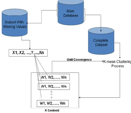
When the missing values in the selected sample are exceeding the number of the available ones, this implies that the measured distance will be in (n-p) space, which means inefficient measured distance. Hence, we will improve the missing values imputation by modifying the steps to obtain the measured distance. When we get the first centroids from the clustering process, we initialize missing values by imputing from prototypes of these centroids. So, the distance measure in the next step becomes in n dimension and, in each new clustering process, imputation will be achieved by measuring the closest distance between whole sample and new centroids. The Modification of Classic Imputation algorithm (MCI) is described as follows: (see Figure 1)
1. Divide data set S into Complete-valued data set St, and Missing-valued data set S∗.
2. Start K-means algorithm on St, while clusters optimized, for each computed centroid wj ,j ∈ {1, 2, ..., k} and
missing-value instance xi , where xi ∈ S∗.Compute distance between centroid wj and missing-value instance xi .
3. Impute missing-value in xi from its corresponding closest centroid wj .
[image:2.595.327.544.76.263.2]4. Repeat step 2 and 3 until k-means convergence.
Fig 1: A Modification of classic Imputation based k-means.
4.
ENHANCEMENT MODIFICATION
OF CLASSIC IMPUTATION METHOD
In each clustering process each sample gets imputed from the centroid of its closest cluster, we count the number of times the sample has been imputed from a particular cluster. The largest number of times a sample gets assigned to a particular cluster means that it belongs to this cluster, which will result in the imputation of the values of the last cluster’s centroid of the most visited cluster to the sample. Enhancement of Modification of Classic Imputation algorithm (EMCI) is described as follow:
1. Divide data set S into Complete-valued data set St, and Missing-valued data set S∗.
2. Initialize class counter C Cj for each missing-value instance, where j ∈ {1, 2, ..., k}.
3. Start K-means algorithm on St, while clusters optimized, for each computed centroid wj , j ∈ {1, 2, ..., k} and
missing-value instance xi , where xi ∈ S∗. Compute distance between centroid wj and missing-value instance xi . 4. Impute missing-value in xi from its corresponding closest centroid wj and increment its corresponding closest center ccj. 5. Repeat step 3 and 4 until k-means convergence. For each missing-value instance xi , where xi ∈ S∗, Choose the maximum class counter and impute missing-value in xi with it is corresponding prototype centroid..
5. EXPERIMENTAL RESULTS
proportional to its cost as more expensive attributes usually have more missing values.
Table 1. Data Sets Used in the Experiments.
Data Base No. of attributes No. of examples
Iris 4 150
Ecoli 7 336
Bupa 6 345
Pima Indian 8 768
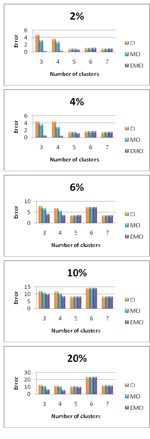
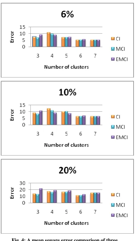
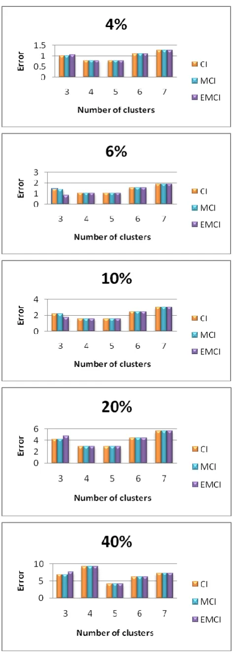
This study shows the performance of three imputation methods based on k-means; Classic Imputation (CI), Modification of Classic Imputation (MCI) and Enhancement of Modification of Classic Imputation (EMCI). Each graph compares the performance of all methods with different level of missing values for different clusters of K-Mean. For the purpose of accuracy, we use the mean square errors which gives from error = (R − I )2 /N where R is real value, I is Imputed value and N is number of missing values.
[image:3.595.63.280.116.181.2]In our experimental results, all figures illustrate the mean square error comparison for the three imputation method describes in previous sections, while all tables illustrate the sum of square errors comparison for simplicity of showing the difference between three methods.
Table 2 illustrates an error comparison between an imputation methods based on k-means, CI, MCI and EMCI in different missing instance percentage at several cluster number for Bupa dataset.
Table 2. A sum of square error comparison of three imputation methods in the Bupa data set.
Miss.(%)
Cluster No Imputation approaches based K-mean CI MCI EMCI
2
3 4 5 6 7
4.777186 3.186759 0.299139 3.581818 2.791975 0.309811 0.907024 0.907024 0.684761 1.116783 1.116783 1.116783
0.95998 0.95998 0.95998
4
3 4 5 6 7
4.383957 3.588674 0.609776 4.39595 2.953905 0.489464 1.481603 1.481604 1.183803 1.669874 1.669874 1.669874 1.527588 1.527589 1.527589 6
3 4 5 6 7
7.765477 6.71576 4.331328 6.907715 5.638264 3.821443 3.641498 3.641498 3.763348 7.375067 7.375067 7.375067 3.671032 3.671032 3.671032 10
3 4 5 6 7
12.01079 11.09118 10.11517 11.92479 10.60073 8.489751 8.332617 8.33262 8.420806 14.09595 14.09595 14.09595
8.28245 8.282451 8.282451 20
3 4 5 6 7
12.76048 11.13619 6.747862 11.67825 10.88445 5.91155 10.84042 10.84041 10.16937 23.74567 23.74565 23.74565 11.98075 11.98074 11.98074
40
3 4 5 6 7
18.34416 16.73777 15.22232 21.26251 20.46837 13.66378 22.84709 22.84707 19.59215 47.41088 47.41081 47.41081 14.56487 14.56487 14.56487
[image:3.595.56.288.434.726.2]Fig. 2: A mean square error comparison of three imputation methods in the Bupa data set.
Table 3. A sum of square error comparison of three imputation methods in the Pima Indian data set.
Miss.(%) Cluster No Imputation approaches based K-mean
CI MCI EMCI
2
3 4 5 6 7 8
14.37554 13.25002 8.890231 13.85666 12.84985 6.06536 13.37925 12.84137 5.971876 11.82608 11.45384 5.877658 5.825113 5.825112 5.916673 7.825108 7.825106 7.825106
4
3 4 5 6 7 8
18.03262 17.36147 13.55296 18.93389 17.38975 12.54147 18.04683 17.85205 12.71843 16.84882 16.74036 11.74633 11.36014 11.36014 11.91438 11.42276 11.42276 11.42276
6
3 4 5 6 7 8
24.44564 23.20973 17.91235 22.63036 21.62001 16.1246 20.38086 20.01029 15.99459 20.81671 20.33147 14.35323 14.01545 14.01545 14.26166 14.28277 14.28277 14.28277
10
3 4 5 6 7 8
38.09534 36.341 33.59278 33.94895 33.3278 29.87464 33.55535 33.02003 30.1552
32.1873 31.36938 27.59835 26.59483 26.59483 27.42991 26.49616 26.49616 26.49616
20
3 4 5 6 7 8
64.64467 62.69846 64.57974 64.20623 63.53032 64.39197 81.72205 81.28112 70.34858 64.43491 63.68247 59.91234 57.20836 57.20828 58.84161 57.41436 57.41428 57.41428
40
3 4 5 6 7 8
[image:4.595.155.540.270.754.2]119.333 117.3868 127.27 119.7724 119.106 127.9656 118.6994 118.2354 127.2739 120.2016 119.4625 117.9062 113.2273 113.2272 115.7847 145.5723 145.5722 145.5722
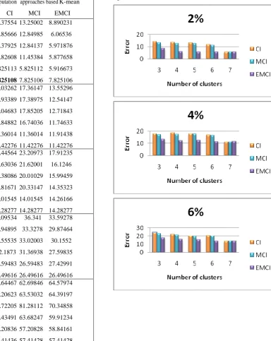
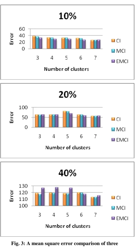
Table 3 illustrates an error comparison between an imputation methods based on k-means, CI, MCI and EMCI in different missing instance percentage at several cluster number for Pima Indian dataset.
Fig. 3: A mean square error comparison of three imputation methods in the Pima Indian data set.
Table 4 illustrates an error comparison between an imputation methods based on k-means, CI, MCI and EMCI in different missing instance percentage at several cluster number for Ecoli data set.
Table 4. A sum of square error comparison of three imputation methods in the Ecoli data set.
Miss.(%) Cluster No
Imputation approaches based K-mean CI MCI EMCI
2
3 4 5 6 7
5.41087 4.531235 4.075765 9.091621 8.014148 3.787097 4.477868 4.462628 3.313772 2.875017 2.875017 3.065405 2.676449 2.676449 2.676449
4
3 4 5 6 7
6.562714 5.990744 6.461079 10.32932 8.963055 6.190022 6.512977 6.551205 5.492534 4.635415 4.635415 5.314992 4.161032 4.161032 4.161032
6
3 4 5 6 7
7.599198 7.035617 9.206245 11.0807 9.722828 8.954317 7.268047 7.306274 7.490683 5.395188 5.395188 5.761791 5.368557 5.368557 5.368557
10
3 4 5 6 7
9.096494 8.35237 10.79339 12.58382 11.04685 9.157546 10.30394 10.36206 8.858151 6.638017 6.638016 7.07966 6.767209 6.767208 6.767208
20
3 4 5 6 7
14.13585 13.38966 22.07389 17.63459 16.09575 19.19012 16.69709 16.76461 18.83994 11.52075 11.52075 13.28862 15.41178 15.41178 15.41178
[image:5.595.310.550.446.715.2]Fig. 4: A mean square error comparison of three imputation methods in the Ecoli data set.
[image:6.595.53.281.584.706.2]Table 5 illustrates an error comparison between an imputation methods based on k-means, CI, MCI and EMCI in different missing instances of percentage at several cluster number for Iris data set.
Table 5. a sum of square error comparison of three imputation methods in the Iris data set.
Miss.(%) Cluster No
Imputation approaches based K-mean CI MCI EMCI
2
3 4 5 6 7
0.447209 0.447209 0.447209 0.420188 0.420188 0.420188 0.420188 0.420188 0.420188 0.457572 0.457572 0.457572 0.536267 0.536267 0.536267
4
3 4 5 6 7
1.018319 1.018319 1.06553 0.790119 0.79012 0.79012 0.790119 0.79012 0.79012 1.105146 1.105146 1.105146 1.278171 1.278171 1.278171
6
3 4 5 6 7
1.438984 1.438984 0.893171 1.066982 1.066982 1.066982 1.066982 1.066982 1.066982 1.588675 1.588675 1.588675 1.926627 1.926627 1.926627
10
3 4 5 6 7
2.252538 2.252538 1.755318 1.629589 1.629589 1.629589 1.629589 1.629589 1.629589 2.499124 2.499124 2.499124 3.06347 3.063469 3.063469
20
3 4 5 6 7
4.289041 4.28904 4.832908 3.045854 3.045854 3.045854 3.045854 3.045854 3.045854 4.535299 4.535299 4.535299 5.684607 5.684606 5.684606
40
3 4 5 6 7
6.942563 6.942573 7.727729 9.3234 9.323404 9.323404 4.254536 4.254535 4.254535 6.270786 6.270789 6.270789 7.323775 7.323776 7.323776
Fig. 5: A mean square error comparison of three imputation methods in the Iris data set.
6.
CONCLUSIONS
Missing data is a usual drawback in many real-world applications. A classical solution is imputation i.e., to estimate and to fill in the unknown values using available data. This work analyzes the behavior of three imputation methods based on k-means; a classic imputation (CI), a modification of classic imputation (MCI) and enhancement of modification of classic imputation (EMCI). The first method (CI) is used and gives higher accuracy than Mean, Mode, Median and c4.5 on dataset such as Bupa, Pima Indian, and e.t. Our proposed methods; (MCI) and (EMCI) is better than the classic (CI). In most cases when the number of clusters is less, the performance of EMCI is better than the two others methods and MCI is better than CI. When the number of clusters is increased the three algorithms are the same.
7.
REFERENCES
[1] Jiawei, H. and Micheline, K., 2006. Data mining Concept and Techniques. 2nd Edn Morgon Kaufmaan Publishers. ISBN: 1-55860-901-6.
[2] Mehala, B., Vivekanandan K. and Ranjit Jeba Thangaiah, P., 2008. An Analysis on K-Means Algorithm as an Imputation Method to Deal with Missing Values. Asian Journal of Information Technology 7 (9): 434-441.
[3] Lakshminarayan, K., Harp, S. A. and Samad, T., 1999. Imputation of missing data in industrial database, Apple. Intell. 11, 259-275.
[4] Jau-Huei Lin and Peter J. Haug, 2008. Exploiting missing clini- cal data in Bayesian network modeling for predicting medical problems Journal of Biomedical Informatics 41, 1-4.
[5] Alireza farhangfar, Lukase Kurgan and Jennifer Dy, 2008. Impact of imputation of missing values on classification error for discrete data. Pattern Recognition 41, 3692-3705.
[6] Dempster, A.P. and LairdandDB Rubin, R. J., 1977. Maximum likelyhood from incomplete data via the EM algoritm (with Discussion). I. R. Stat. Soc, B39: 1-38. http://wwwjstororg/pss/2984875.
[7] Daqian, G. and Yang, G. 2005. Incremental gradent descent imputation method for missing data in learning classifier systems. GECCO, ACM, Wash- ington, DC, USA, pp: 72-73.
[8] Fulufhelo, V., Nelwamondo and Tshlidzi, M. 2007. Rough sets computations to impute missing data. Comput. Vision and Pattern Recog., 1, 1-19.
[9] Musil, C.M., Wamer, C.B., Yobas , P.K. and Jones, S.L. 2002. A comparison of imputation techniques for han- dling missing data. Western J. Nus. Res., 24 (5).
[10]Cristian P., D., Alain, P. Monique and Tahar, K. 2005. Tools for statistical analysis with missing data: Appli cation to a large medxal database. ENMI, pp: 181-186. [11]Joseph L. Schafer and Maren K. Olsen, 1998. Multiple
Imputation for multivariate Missing data problems: a data analyst's perspective, 33, 545--571.
Classification and missing data imputation. Neurocomputing 72, 1483-1493.
[13]Allison, P. D., 2001. Missing data, Sage University Papers Serieson Quantitative Applications in the Social Sciences, Thousand Oaks, California, USA.
[14]Little, R. J. A. and Rubin, D. B. Statistical 2002. Analysis with Missing Data, seconded, Wiley, NJ, USA. [15]Sande, G. 1983. Hot Deck Imputation Procedures,